Routing
William Stallings Data and Computer Communications 7 th Edition (Selected slides used for lectures at Bina Nusantara University). Routing. Routing in Circuit Switched Network. Many connections will need paths through more than one switch Need to find a route Efficiency Resilience

Routing
E N D
Presentation Transcript
William StallingsData and Computer Communications7th Edition(Selected slides used for lectures at Bina Nusantara University) Routing
Routing in Circuit Switched Network • Many connections will need paths through more than one switch • Need to find a route • Efficiency • Resilience • Public telephone switches are a tree structure • Static routing uses the same approach all the time • Dynamic routing allows for changes in routing depending on traffic • Uses a peer structure for nodes
Alternate Routing • Possible routes between end offices predefined • Originating switch selects appropriate route • Routes listed in preference order • Different sets of routes may be used at different times
Routing in Packet Switched Network • Complex, crucial aspect of packet switched networks • Characteristics required • Correctness • Simplicity • Robustness • Stability • Fairness • Optimality • Efficiency
Performance Criteria • Used for selection of route • Minimum hop • Least cost • See Stallings appendix 10A for routing algorithms
Decision Time and Place • Time • Packet or virtual circuit basis • Place • Distributed • Made by each node • Centralized • Source
Network Information Source and Update Timing • Routing decisions usually based on knowledge of network (not always) • Distributed routing • Nodes use local knowledge • May collect info from adjacent nodes • May collect info from all nodes on a potential route • Central routing • Collect info from all nodes • Update timing • When is network info held by nodes updated • Fixed - never updated • Adaptive - regular updates
Routing Strategies • Fixed • Flooding • Random • Adaptive
Fixed Routing • Single permanent route for each source to destination pair • Determine routes using a least cost algorithm (appendix 10A) • Route fixed, at least until a change in network topology
Flooding • No network info required • Packet sent by node to every neighbor • Incoming packets retransmitted on every link except incoming link • Eventually a number of copies will arrive at destination • Each packet is uniquely numbered so duplicates can be discarded • Nodes can remember packets already forwarded to keep network load in bounds • Can include a hop count in packets
Properties of Flooding • All possible routes are tried • Very robust • At least one packet will have taken minimum hop count route • Can be used to set up virtual circuit • All nodes are visited • Useful to distribute information (e.g. routing)
Random Routing • Node selects one outgoing path for retransmission of incoming packet • Selection can be random or round robin • Can select outgoing path based on probability calculation • No network info needed • Route is typically not least cost nor minimum hop
Adaptive Routing • Used by almost all packet switching networks • Routing decisions change as conditions on the network change • Failure • Congestion • Requires info about network • Decisions more complex • Tradeoff between quality of network info and overhead • Reacting too quickly can cause oscillation • Too slowly to be relevant
Adaptive Routing - Advantages • Improved performance • Aid congestion control (See chapter 13) • Complex system • May not realize theoretical benefits
Classification • Based on information sources • Local (isolated) • Route to outgoing link with shortest queue • Can include bias for each destination • Rarely used - do not make use of easily available info • Adjacent nodes • All nodes
ARPANET Routing Strategies(1) • First Generation • 1969 • Distributed adaptive • Estimated delay as performance criterion • Bellman-Ford algorithm (appendix 10a) • Node exchanges delay vector with neighbors • Update routing table based on incoming info • Doesn't consider line speed, just queue length • Queue length not a good measurement of delay • Responds slowly to congestion
ARPANET Routing Strategies(2) • Second Generation • 1979 • Uses delay as performance criterion • Delay measured directly • Uses Dijkstra’s algorithm (appendix 10a) • Good under light and medium loads • Under heavy loads, little correlation between reported delays and those experienced
ARPANET Routing Strategies(3) • Third Generation • 1987 • Link cost calculations changed • Measure average delay over last 10 seconds • Normalize based on current value and previous results
Least Cost Algorithms • Basis for routing decisions • Can minimize hop with each link cost 1 • Can have link value inversely proportional to capacity • Given network of nodes connected by bi-directional links • Each link has a cost in each direction • Define cost of path between two nodes as sum of costs of links traversed • For each pair of nodes, find a path with the least cost • Link costs in different directions may be different • E.g. length of packet queue
Dijkstra’s Algorithm Definitions • Find shortest paths from given source node to all other nodes, by developing paths in order of increasing path length • N= set of nodes in the network • s = source node • T= set of nodes so far incorporated by the algorithm • w(i, j)= link cost from node i to node j • w(i, i) = 0 • w(i, j) = if the two nodes are not directly connected • w(i, j) 0 if the two nodes are directly connected • L(n)=cost of least-cost path from node s to node n currently known • At termination, L(n) is cost of least-cost path from s to n
Dijkstra’s Algorithm Method • Step 1 [Initialization] • T = {s} Set of nodes so far incorporated consists of only source node • L(n) = w(s, n) for n ≠ s • Initial path costs to neighboring nodes are simply link costs • Step 2[Get Next Node] • Find neighboring node not in T with least-cost path from s • Incorporate node into T • Also incorporate the edge that is incident on that node and a node in T that contributes to the path • Step 3[Update Least-Cost Paths] • L(n) = min[L(n), L(x) + w(x, n)]for all nÏ T • If latter term is minimum, path from s to n is path from s to x concatenated with edge from x to n • Algorithm terminates when all nodes have been added to T
Dijkstra’s Algorithm Notes • At termination, value L(x) associated with each node x is cost (length) of least-cost path from s to x. • In addition, T defines least-cost path from s to each other node • One iteration of steps 2 and 3 adds one new node to T • Defines least cost path from s tothat node
Bellman-Ford Algorithm Definitions • Find shortest paths from given node subject to constraint that paths contain at most one link • Find the shortest paths with a constraint of paths of at most two links • And so on • s = source node • w(i, j)=link cost from node i to node j • w(i, i) = 0 • w(i, j) = if the two nodes are not directly connected • w(i, j) 0 if the two nodes are directly connected • h = maximum number of links in path at current stage of the algorithm • Lh(n)=cost of least-cost path from s to n under constraint of no more than h links
Bellman-Ford Algorithm Method • Step 1 [Initialization] • L0(n) = , for all n s • Lh(s) = 0, for all h • Step 2 [Update] • For each successive h 0 • For each n ≠ s, compute • Lh+1(n)=minj[Lh(j)+w(j,n)] • Connect n with predecessor node j that achieves minimum • Eliminate any connection of n with different predecessor node formed during an earlier iteration • Path from s to n terminates with link from j to n
Bellman-Ford Algorithm Notes • For each iteration of step 2 with h=K and for each destination node n, algorithm compares paths from s to n of length K=1 with path from previous iteration • If previous path shorter it is retained • Otherwise new path is defined
Comparison • Results from two algorithms agree • Information gathered • Bellman-Ford • Calculation for node n involves knowledge of link cost to all neighboring nodes plus total cost to each neighbor from s • Each node can maintain set of costs and paths for every other node • Can exchange information with direct neighbors • Can update costs and paths based on information from neighbors and knowledge of link costs • Dijkstra • Each node needs complete topology • Must know link costs of all links in network • Must exchange information with all other nodes
Evaluation • Dependent on processing time of algorithms • Dependent on amount of information required from other nodes • Implementation specific • Both converge under static topology and costs • Converge to same solution • If link costs change, algorithms will attempt to catch up • If link costs depend on traffic, which depends on routes chosen, then feedback • May result in instability
Routing Protocols • Routing Information • About topology and delays in the internet • Routing Algorithm • Used to make routing decisions based on information
Autonomous Systems (AS) • Group of routers • Exchange information • Common routing protocol • Set of routers and networks managed by signle organization • A connected network • There is at least one route between any pair of nodes
Interior Router Protocol (IRP)Exterior Routing Protocol (ERP) • Passes routing information between routers within AS • May be more than one AS in internet • Routing algorithms and tables may differ between different AS • Routers need some info about networks outside their AS • Used exterior router protocol (ERP) • IRP needs detailed model • ERP supports summary information on reachability
Approaches to Routing – Distance-vector • Each node (router or host) exchange information with neighboring nodes • Neighbors are both directly connected to same network • First generation routing algorithm for ARPANET • Node maintains vector of link costs for each directly attached network and distance and next-hop vectors for each destination • Used by Routing Information Protocol (RIP) • Requires transmission of lots of information by each router • Distance vector to all neighbors • Contains estimated path cost to all networks in configuration • Changes take long time to propagate
Approaches to Routing – Link-state • Designed to overcome drawbacks of distance-vector • When router initialized, it determines link cost on each interface • Advertises set of link costs to all other routers in topology • Not just neighboring routers • From then on, monitor link costs • If significant change, router advertises new set of link costs • Each router can construct topology of entire configuration • Can calculate shortest path to each destination network • Router constructs routing table, listing first hop to each destination • Router does not use distributed routing algorithm • Use any routing algorithm to determine shortest paths • In practice, Dijkstra's algorithm • Open shortest path first (OSPF) protocol uses link-state routing. • Also second generation routing algorithm for ARPANET
Exterior Router Protocols –Not Distance-vector • Link-state and distance-vector not effective for exterior router protocol • Distance-vector assumes routers share common distance metric • ASs may have different priorities • May have restrictions that prohibit use of certain other AS • Distance-vector gives no information about ASs visited on route
Exterior Router Protocols –Not Link-state • Different ASs may use different metrics and have different restrictions • Impossible to perform a consistent routing algorithm. • Flooding of link state information to all routers unmanageable
Exterior Router Protocols –Path-vector • Dispense with routing metrics • Provide information about which networks can be reached by a given router and ASs crossed to get there • Does not includedistance or cost estimate • Each block of information lists all ASs visited on this route • Enables router to perform policy routing • E.g. avoid path to avoid transiting particular AS • E.g. link speed, capacity, tendency to become congested, and overall quality of operation, security • E.g. minimizing number of transit ASs
Open Shortest Path First (1) • OSPF • IGP of Internet • Replaced Routing Information Protocol (RIP) • Uses Link State Routing Algorithm • Each router keeps list of state of local links to network • Transmits update state info • Little traffic as messages are small and not sent often • RFC 2328 • Route computed on least cost based on user cost metric
Open Shortest Path First (2) • Topology stored as directed graph • Vertices or nodes • Router • Network • Transit • Stub • Edges • Graph edge • Connect two router • Connect router to network
Operation • Dijkstra’s algorithm used to find least cost path to all other networks • Next hop used in routing packets