Routing

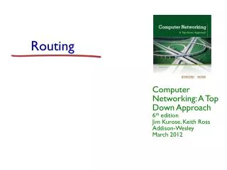
1. Routing Computer Networking: A Top Down Approach 6th edition Jim Kurose, Keith RossAddison-WesleyMarch 2012

2. routing algorithm local forwarding table header value output link 0100 0101 0111 1001 3 2 2 1 value in arriving packet’s header 1 0111 2 3 Interplay between routing, forwarding

3. 5 3 5 2 2 1 3 1 2 1 x z w u y v Graph abstraction Graph: G = (N,E) N = set of routers = { u, v, w, x, y, z } E = set of links ={ (u,v), (u,x), (v,x), (v,w), (x,w), (x,y), (w,y), (w,z), (y,z) } Remark: Graph abstraction is useful in other network contexts Example: P2P, where N is set of peers and E is set of TCP connections

4. 5 3 5 2 2 1 3 1 2 1 x z w u y v Graph abstraction: costs • c(x,x’) = cost of link (x,x’) - e.g., c(w,z) = 5 • cost could always be 1, or inversely related to bandwidth, or inversely related to congestion Cost of path (x1, x2, x3,…, xp) = c(x1,x2) + c(x2,x3) + … + c(xp-1,xp) Question: What’s the least-cost path between u and z ? Routing algorithm: algorithm that finds least-cost path

5. Global or decentralized information? Global: all routers have complete topology, link cost info “link state” algorithms Decentralized: router knows physically-connected neighbors, link costs to neighbors iterative process of computation, exchange of info with neighbors “distance vector” algorithms Static or dynamic? Static: routes change slowly over time Dynamic: routes change more quickly periodic update in response to link cost changes Routing Algorithm classification

6. Dijkstra’s algorithm net topology, link costs known to all nodes accomplished via “link state broadcast” all nodes have same info computes least cost paths from one node (‘source”) to all other nodes gives forwarding table for that node iterative: after k iterations, know least cost path to k dest.’s Notation: c(x,y): link cost from node x to y; = ∞ if not direct neighbors D(v): current value of cost of path from source to dest. v p(v): predecessor node along path from source to v N': set of nodes whose least cost path definitively known A Link-State Routing Algorithm

7. Dijsktra’s Algorithm 1 Initialization: 2 N' = {u} 3 for all nodes v 4 if v adjacent to u 5 then D(v) = c(u,v) 6 else D(v) = ∞ 7 8 Loop 9 find w not in N' such that D(w) is a minimum 10 add w to N' 11 update D(v) for all v adjacent to w and not in N' : 12 D(v) = min( D(v), D(w) + c(w,v) ) 13 /* new cost to v is either old cost to v or known 14 shortest path cost to w plus cost from w to v */ 15 until all nodes in N'

8. 5 3 5 2 2 1 3 1 2 1 x z w y u v Dijkstra’s algorithm: example D(v),p(v) 2,u 2,u 2,u D(x),p(x) 1,u D(w),p(w) 5,u 4,x 3,y 3,y D(y),p(y) ∞ 2,x Step 0 1 2 3 4 5 N' u ux uxy uxyv uxyvw uxyvwz D(z),p(z) ∞ ∞ 4,y 4,y 4,y

9. x z w u y v destination link (u,v) v (u,x) x y (u,x) (u,x) w z (u,x) Dijkstra’s algorithm: example (2) Resulting shortest-path tree from u: Resulting forwarding table in u:

10. Dijkstraalgorithm illustration 5 a [2 / s] b [5 / s] 3 2 4 e s 3 2 1 2 [∞ / ] [0 / s] 1 1 c d [∞ / ] [1 / s]

11. Dijkstraalgorithm illustration 5 a [2 / s] b [4 / c] 3 2 4 e s 3 2 1 2 [∞ / ] [0 / s] 1 1 c d [2 / c] [1 / s]

12. Dijkstraalgorithm illustration 5 a [2 / s] b [4 / c] 3 2 4 e s 3 2 1 2 [∞ / ] [0 / s] 1 1 c d [2 / c] [1 / s]

13. Dijkstraalgorithm illustration 5 a [2 / s] b [3 / d] 3 2 4 e s 3 2 1 2 [4 / d] [0 / s] 1 1 c d [2 / c] [1 / s]

14. Dijkstraalgorithm illustration 5 a [2 / s] b [3 / d] 3 2 4 e s 3 2 1 2 [4 / d] [0 / s] 1 1 c d [2 / c] [1 / s]

15. Dijkstraalgorithm illustration 5 a [2 / s] b [3 / d] 3 2 4 e s 3 2 1 2 [4 / d] [0 / s] 1 1 c d [2 / c] [1 / s]

16. a b s e c d Dijkstraalgorithm summary • 复杂度 (Complexity) – O(n2) 注意: 计算所有的最短路径和计算一条最短路径具有相同的复杂度。 • 输出结果给出了网络上的一棵生成树 (Spanning Tree)。 5 3 2 4 3 2 1 1 2 1

17. Algorithm complexity: n nodes each iteration: need to check all nodes, w, not in N n(n+1)/2 comparisons: O(n2) more efficient implementations possible: O(nlogn) Oscillations possible: e.g., link cost = amount of carried traffic A A A A D D D D B B B B C C C C 1 1+e 2+e 0 2+e 0 2+e 0 0 0 1 1+e 0 0 1 1+e e 0 0 0 e 1 1+e 0 1 1 e … recompute … recompute routing … recompute initially Dijkstra’s algorithm, discussion

18. Distance Vector Algorithm Bellman-Ford Equation (dynamic programming) Define dx(y) := cost of least-cost path from x to y Then dx(y) = min {c(x,v) + dv(y) } where min is taken over all neighbors v of x v

19. 5 3 5 2 2 1 3 1 2 1 x z w u y v Bellman-Ford example Clearly, dv(z) = 5, dx(z) = 3, dw(z) = 3 B-F equation says: du(z) = min { c(u,v) + dv(z), c(u,x) + dx(z), c(u,w) + dw(z) } = min {2 + 5, 1 + 3, 5 + 3} = 4 Node that achieves minimum is next hop in shortest path ➜ forwarding table

20. Distance Vector Algorithm • Dx(y) = estimate of least cost from x to y • Node x knows cost to each neighbor v: c(x,v) • Node x maintains distance vector Dx = [Dx(y): y є N ] • Node x also maintains its neighbors’ distance vectors • For each neighbor v, x maintains Dv = [Dv(y): y є N ]

21. Distance vector algorithm (4) Basic idea: • From time-to-time, each node sends its own distance vector estimate to neighbors • Asynchronous • When a node x receives new DV estimate from neighbor, it updates its own DV using B-F equation: Dx(y) ← minv{c(x,v) + Dv(y)} for each node y ∊ N • Under minor, natural conditions, the estimate Dx(y) converge to the actual least costdx(y)

22. Iterative, asynchronous: each local iteration caused by: local link cost change DV update message from neighbor Distributed: each node notifies neighbors only when its DV changes neighbors then notify their neighbors if necessary wait for (change in local link cost or msg from neighbor) recompute estimates if DV to any dest has changed, notify neighbors Distance Vector Algorithm (5) Each node:

23. cost to x y z x 0 2 7 y from ∞ ∞ ∞ z ∞ ∞ ∞ 2 1 7 z x y Dx(z) = min{c(x,y) + Dy(z), c(x,z) + Dz(z)} = min{2+1 , 7+0} = 3 Dx(y) = min{c(x,y) + Dy(y), c(x,z) + Dz(y)} = min{2+0 , 7+1} = 2 node x table cost to x y z x 0 2 3 y from 2 0 1 z 7 1 0 node y table cost to x y z x ∞ ∞ ∞ 2 0 1 y from z ∞ ∞ ∞ node z table cost to x y z x ∞ ∞ ∞ y from ∞ ∞ ∞ z 7 1 0 time

24. cost to x y z x 0 2 7 y from ∞ ∞ ∞ z ∞ ∞ ∞ 2 1 7 z x y Dx(z) = min{c(x,y) + Dy(z), c(x,z) + Dz(z)} = min{2+1 , 7+0} = 3 Dx(y) = min{c(x,y) + Dy(y), c(x,z) + Dz(y)} = min{2+0 , 7+1} = 2 node x table cost to cost to x y z x y z x 0 2 3 x 0 2 3 y from 2 0 1 y from 2 0 1 z 7 1 0 z 3 1 0 node y table cost to cost to cost to x y z x y z x y z x ∞ ∞ x 0 2 7 ∞ 2 0 1 x 0 2 3 y y from 2 0 1 y from from 2 0 1 z z ∞ ∞ ∞ 7 1 0 z 3 1 0 node z table cost to cost to cost to x y z x y z x y z x 0 2 7 x 0 2 3 x ∞ ∞ ∞ y y 2 0 1 from from y 2 0 1 from ∞ ∞ ∞ z z z 3 1 0 3 1 0 7 1 0 time

25. 1 4 1 50 x z y Distance Vector: link cost changes Link cost changes: • node detects local link cost change • updates routing info, recalculates distance vector • if DV changes, notify neighbors At time t0, y detects the link-cost change, updates its DV, and informs its neighbors. “good news travels fast” At time t1, z receives the update from y and updates its table. It computes a new least cost to x and sends its neighbors its DV. At time t2, y receives z’s update and updates its distance table. y’s least costs do not change and hence y does not send any message to z.

26. X Z Y Distance Vector: link cost changes 1 Good news spreads fast 4 1 50 算法 收敛

27. 60 4 1 50 x z y Distance Vector: link cost changes Link cost changes: • good news travels fast • bad news travels slow - “count to infinity” problem! • 44 iterations before algorithm stabilizes: see text Poisoned reverse: • If Z routes through Y to get to X : • Z tells Y its (Z’s) distance to X is infinite (so Y won’t route to X via Z) • will this completely solve count to infinity problem?

28. X Z Y Distance Vector: link cost changes Bad news spreads slowly, so called “Count to Infinity Problem”: 60 4 1 50 算法仍 不收敛

29. X Z Y Distance Vector–Poisoned Reverse Poisoned Reverse:如果 Z 到 X 的最短路径经过 Y，那么 Z 告诉 Y “Z 到 X 的最短距离是 ∞ “，这样 Y 就不会选择经由 Z 到达 X 的路线。 60 4 1 50 算法 收敛 ∞ 立即修改

30. Message complexity LS: with n nodes, E links, O(nE) msgs sent DV: exchange between neighbors only convergence time varies Speed of Convergence LS: O(n2) algorithm requires O(nE) msgs may have oscillations DV: convergence time varies may be routing loops count-to-infinity problem Robustness: what happens if router malfunctions? LS: node can advertise incorrect link cost each node computes only its own table DV: DV node can advertise incorrect path cost each node’s table used by others error propagate thru network Comparison of LS and DV algorithms

31. DV versus LS Distance Vector Link State • 仅与邻居节点交换消息 • 消息包括到所有节点的最短距离 • 收敛速度比较慢 • 能够广播不正确的路径信息 • 有Count to Infinity Problem • 向网络上所有其它节点广播消息 • 消息仅包括到邻居节点的距离 • 收敛速度比较快 • 能够广播不正确的链路信息 • 没有Count to Infinity Problem

32. scale: with 200 million destinations: can’t store all dest’s in routing tables! routing table exchange would swamp links! administrative autonomy internet = network of networks each network admin may want to control routing in its own network Hierarchical Routing Our routing study thus far - idealization • all routers identical • network “flat” … not true in practice

33. aggregate routers into regions, “autonomous systems” (AS) routers in same AS run same routing protocol “intra-AS” routing protocol routers in different AS can run different intra-AS routing protocol Gateway router Direct link to router in another AS Hierarchical Routing

34. forwarding table configured by both intra- and inter-AS routing algorithm intra-AS sets entries for internal dests inter-AS & intra-As sets entries for external dests 3a 3b 2a AS3 AS2 1a 2c AS1 2b 3c 1b 1d 1c Inter-AS Routing algorithm Intra-AS Routing algorithm Forwarding table Interconnected ASes

35. suppose router in AS1 receives datagram destined outside of AS1: router should forward packet to gateway router, but which one? AS1 must: learn which dests are reachable through AS2, which through AS3 propagate this reachability info to all routers in AS1 Job of inter-AS routing! 3a 3b 2a AS3 AS2 1a AS1 2c 2b 3c 1b 1d 1c Inter-AS tasks

36. 2c 2b 3c 1b 1d 1c Example: Setting forwarding table in router 1d • suppose AS1 learns (via inter-AS protocol) that subnet x reachable via AS3 (gateway 1c) but not via AS2. • inter-AS protocol propagates reachability info to all internal routers. • router 1d determines from intra-AS routing info that its interface I is on the least cost path to 1c. • installs forwarding table entry (x,I) … x 3a 3b 2a AS3 AS2 1a AS1

37. 3a 3b 2a AS3 AS2 1a AS1 2c 2b 3c 1b 1d 1c Example: Choosing among multiple ASes • now suppose AS1 learns from inter-AS protocol that subnet x is reachable from AS3 and from AS2. • to configure forwarding table, router 1d must determine towards which gateway it should forward packets for dest x. • this is also job of inter-AS routing protocol! … … x

38. Determine from forwarding table the interface I that leads to least-cost gateway. Enter (x,I) in forwarding table Use routing info from intra-AS protocol to determine costs of least-cost paths to each of the gateways Learn from inter-AS protocol that subnet x is reachable via multiple gateways Hot potato routing: Choose the gateway that has the smallest least cost Example: Choosing among multiple ASes • now suppose AS1 learns from inter-AS protocol that subnet x is reachable from AS3 and from AS2. • to configure forwarding table, router 1d must determine towards which gateway it should forward packets for dest x. • this is also job of inter-AS routing protocol! • hot potato routing: send packet towards closest of two routers.

39. Intra-AS Routing • also known as Interior Gateway Protocols (IGP) • most common Intra-AS routing protocols: • RIP: Routing Information Protocol • OSPF: Open Shortest Path First • IGRP: Interior Gateway Routing Protocol (Cisco proprietary)

40. u v destinationhops u 1 v 2 w 2 x 3 y 3 z 2 w x z y C A D B RIP ( Routing Information Protocol) • distance vector algorithm • included in BSD-UNIX Distribution in 1982 • distance metric: # of hops (max = 15 hops) From router A to subnets:

41. RIP advertisements • distance vectors: exchanged among neighbors every 30 sec via Response Message (also called advertisement) • each advertisement: list of up to 25 destination subnets within AS

42. RIP: Example z w x y A D B C Destination Network Next Router Num. of hops to dest. w A 2 y B 2 z B 7 x -- 1 …. …. .... Routing/Forwarding table in D

43. z w x y A D B C RIP: Example Dest Next hops w - 1 x - 1 z C 4 …. … ... Advertisement from A to D Destination Network Next Router Num. of hops to dest. w A 2 y B 2 z B A 7 5 x -- 1 …. …. .... Routing/Forwarding table in D

44. RIP: Link Failure and Recovery If no advertisement heard after 180 sec --> neighbor/link declared dead • routes via neighbor invalidated • new advertisements sent to neighbors • neighbors in turn send out new advertisements (if tables changed) • link failure info quickly (?) propagates to entire net • poison reverse used to prevent ping-pong loops (infinite distance = 16 hops)

45. routed routed RIP Table processing • RIP routing tables managed by application-level process called route-d (daemon) • advertisements sent in UDP packets, periodically repeated Transprt (UDP) Transprt (UDP) network forwarding (IP) table network (IP) forwarding table link link physical physical

46. OSPF (Open Shortest Path First) • “open”: publicly available • uses Link State algorithm • LS packet dissemination • topology map at each node • route computation using Dijkstra’s algorithm • OSPF advertisement carries one entry per neighbor router • advertisements disseminated to entire AS (via flooding) • carried in OSPF messages directly over IP (rather than TCP or UDP

47. OSPF “advanced” features (not in RIP) • security: all OSPF messages authenticated (to prevent malicious intrusion) • multiple same-cost paths allowed (only one path in RIP) • For each link, multiple cost metrics for different TOS (e.g., satellite link cost set “low” for best effort; high for real time) • integrated uni- and multicast support: • Multicast OSPF (MOSPF) uses same topology data base as OSPF • hierarchical OSPF in large domains.

48. Hierarchical OSPF

49. Hierarchical OSPF • two-level hierarchy: local area, backbone. • Link-state advertisements only in area • each nodes has detailed area topology; only know direction (shortest path) to nets in other areas. • area border routers:“summarize” distances to nets in own area, advertise to other Area Border routers. • backbone routers: run OSPF routing limited to backbone. • boundary routers: connect to other AS’s.

50. Internet inter-AS routing: BGP • BGP (Border Gateway Protocol):the de facto standard • BGP provides each AS a means to: • Obtain subnet reachability information from neighboring ASs. • Propagate reachability information to all AS-internal routers. • Determine “good” routes to subnets based on reachability information and policy. • allows subnet to advertise its existence to rest of Internet: “I am here”