Routing
Routing. Connectionless Network Layers. Destination, source, hop count Maybe other stuff fragmentation options (e.g., source routing) error reports special service requests (priority, custom routes) congestion indication Real diff: size of addresses. Comparative Addresses.

Routing
E N D
Presentation Transcript
Connectionless Network Layers • Destination, source, hop count • Maybe other stuff • fragmentation • options (e.g., source routing) • error reports • special service requests (priority, custom routes) • congestion indication • Real diff: size of addresses
Comparative Addresses • IPv4: 4 bytes, boundary depends on “mask” • IPX: 10 bytes: 4=link, 6=node • AppleTalk: 2=link, 1=node • CLNP: variable length, 14=“area”, 6=node • IPv6: 16 bytes: 8=link, 8=node (?)
IPv4 data packet version hdr lnth TOS total length 2 pkt id 2 df mf offset offset (cont’d) Don’t Fragment More Fragments TTL (time to live) protocol hdr checksum 2 4 source TCP, UDP 4 destination options variable variable padding
IPv6 vers TOS flow label (20 bits) (4 bits) (8 bits) payload length next hops remain source destination hop by hop hdr, or rtg hdr, or authentication hdr, or end-to-end, or TCP, or ...
Distributed Routing Protocols • Rtrs exchange control info • Use it to calculate forwarding table • Two basic types • distance vector (DECnet, “old” ARPANET, RIP) • link state (“new” ARPANET 1980,DECnet Phase V 1985, IS-IS 1988, OSPF version 2 1998).
cost 2 j m cost 3 I am “4” cost 7 cost 2 k n Distance Vector Routing • Rtr knows • own ID • how many cables hanging off box • cost, for each cable, of getting to nbr
Distance Vector (DV) Routing • Initialize distances to all rtrs in the network to be 0, except to its nbrs. • Rtr learns from nbrs their distances to all nodes in the network, calculate own distances, and forward the distance vector to nbrs. This repeats until the distance vector converges. • Rtr updates the distance vector whenever it receives different distance vector from some nbr, or whenever some link breaks. • Distance vector is either sent periodically or when the network configuration changes.
Example of DV Routing cost 2 j m cost 3 I am “4” cost 7 cost 2 k n distance vector rcv’d from cable j cost 3 12 3 15 3 12 5 3 18 0 7 15 distance vector rcv’d from cable k cost 2 5 8 3 2 10 7 4 20 5 0 15 distance vector rcv’d from cable m cost 2 0 5 3 2 19 9 5 22 2 4 7 distance vector rcv’d from cable n cost 7 6 2 0 7 8 5 8 12 11 3 2 your own calculated distance vector 2 6 5 0 12 8 6 19 3 ? ? your own calculated forwarding table m j m 0 k j k/j n j ? ?
A B C Problems with Distance Vector Routing • B does not conclude that C is unreachable but that d(B,C)=d(B,A)+d(A,C) =3 • When A receives DV from B it concludes that d(A,C)=4 • DV increases in this until infinity, or maximum value which is set by administrator. For this reason, the cost field has the small size.
R1 R2 D Split Horizon • This technique sometime prevents counting toward infinity. • If R1 forwards packetsto D through R2, then R2 informs R1 that its distance to D is infinity. • So, when the link toward node D fails, R2 concludes that its distance to D is infinity immediately, i.e. that D is unreachable.
R2 R3 R1 D Split Horizon • Unfortunatelly, split horizon does not always work. • When link to D fails, R1 concludes that D is unreachable. • R2 gets the information from R1 that D is unreachable, and sets the path to D through R2, calculating DV based on DC of R2, and vice versa.
Link State Routing • Construct Link State Packet (LSP) • who you are • list of (nbr, cost) pairs • Broadcast LSPs to all rtrs • Store latest LSP from each rtr received from nbrs • Compute Routes • Forward LSPs from each nbr to other nbrs
Building Link State Packets (a) A subnet. (b) The link state packets for this subnet.
Broadcasting LSP • LSPs are distributed through flooding • send to every nbr except from which LSP rcv’d • LSP is updated only if it has a higher sequence number than the existing one, or if its age exceeded the maximum age. • Rtr forwards only updated LSPs, and it generates new LSPs periodically or when there is a configuration change (link cost has changed, nbr is down).
Fixing the Algorithm • Require LSPs to age at every hop • Make sequence number large and linear • Careful synchronization between nbrs • At most one LSP from one source • Each LSP has flags for acknowledgements and transmissions to nbrs. • When LSP is received from some nbr its corresponding ack flag is set, as well as its send flags to other nbrs. • Acknowledgments for LSP reception from one nbr are sent to it in a round-robin fashion. LSPs with the send flags for some nbr set, are sent to it also in a round-robin fashion.
Arithmetic in Circular Space • Sequence number a is smaller than sequence number b when it holds:
Distributing the Link State Packets The packet buffer for router B in the previous slide (Fig. 5-13).
Computing Routes • Edsgar Dijkstra’s algorithm: • calculate tree of shortest paths from self to each • also calculate cost from self to each • Algorithm: • step 0: put (SELF, 0) on tree • step 1: look at LSP of node (N,c) just put on tree. If for any nbr K, this is best path so far to K, put (K, c+dist(N,K)) on tree, child of N, with dotted line • step 2: make dotted line with smallest cost solid, go to step 1
6 2 A B C 5 2 2 1 G 2 4 D E F 1 A B C D E F G B/6 A/6 B/2 A/2 B/1 C/2 C/5 D/2 C/2 F/2 E/2 D/2 E/4 F/1 E/1 G/5 F/4 G/1 Example of Dijkstra Algorithm
C(0) C(0) C(0) B(2) G(5) B(2) G(5) B(2) G(5) F(2) F(2) F(2) E(6) G(3) C(0) C(0) C(0) B(2) B(2) B(2) F(2) A(8) E(3) F(2) A(8) E(3) F(2) E(6) G(3) E(6) G(3) G(3) Example of Dijkstra Algorithm
C(0) C(0) C(0) B(2) B(2) B(2) A(8) E(3) F(2) A(8) E(3) F(2) A(8) E(3) F(2) D(5) D(5) D(5) G(3) G(3) G(3) A(7) C(0) B(2) E(3) F(2) D(5) G(3) A(7) Example of Dijkstra Algorithm Forwarding table: A/B B/B C/self D/B E/B F/F G/F
Distance Vector vs Link State • Memory: distance vector wins (but memory is cheap) • Computation: debatable • Simplicity of coding: simple distance vector wins. • Convergence speed: link state better • Functionality: link state can have custom routes, mapping the net, easier troubleshooting,
Specific Routing Protocols • Interdomain vs Intradomain • Intradomain: link state (OSPF, IS-IS) vs distance vector (RIP) • Interdomain • static routing • EGP • BGP • ?
Routing Information Protocol (RIP) • Packets are requests and responses. • Report through response every destination every 30 seconds, or as a reply to request. • Throw away info if too old (90? for IP) • Request when a rtr comes up or when info is too old • Maximum cost is 16 • Most implementations of IP RIP do • split horizon • triggered updates • poison reverse (rtr that learns about link fail announce the distance through it as infinity).
Link State Routing Protocols • Intermediate system-intermediate system (IS-IS) is ISO standard; Netware link state protocol (NLSP) is modification of IS-IS; Private network-to-network interface (PNNI) for ATM; Open shortest path first (OSPF); • Similarities and differences: hierarchy, area addresses, LANs, parameter synchronization, number of destinations per LSP, LSP database overload, authentication.
IS-IS Pkt Types • Hello • pt-to-pt • LAN (extra stuff like LAN name, 2-way connectivity check) • Sequence number packet (SNP) • CSNP (complete), for LAN sync, and startup • PSNP (partial), for acking one or more LSPs • LSPs.
OSPF Pkt Types • Hellos • Database description • Startup • Link state request • Link state update • Multiple LSAs • Link state ack • Links state advertisement (LSA) • type 1 LSA (like IS-IS ordinary LSP) • type 2 LSA (like IS-IS LSP on a LAN) • types 3, 4, 5, … external info
OSPF types 3, 4, and 5 LSAs area border router IP prefix AS border rtr 3 AS 3 3 area 5 3 5 4 4 5
OSPF • Runs on the top of IP with protocol field 89. • Comprises two levels of hierarchy: areas and backbone. • Boarder routers of some domain calculate their costs to the destinations outside the domain and flood the information into the area, so that area routers can calculate optimal path.
OSPF • Hierarchy: OSPF has two levels of hierarchy. Boarder routers of any area calculate their costs to the boarder routers of the autonomous system (AS) and inject those to the area. The AS boarder routers report their cost to the destinations outside of the area. • Area addresses: area has ID (4 bajta), where 0.0.0.0 denotes level 2 in hierarchy. No possibility for dynamic merging or splitting the areas.
OSPF • Routing in LAN: DR expects an acknowledgment from LAN routers for each link stage advertisement (LSA). A backup DR (BDR) keeps the replicated LSA database. Whenever some LAN router sends LSA it multicasts it to DR and BDR. Acks are also multicast to DR and BDR. If there is no ack, LSA is sent to the individual router. • Parameter sync.: HelloInterval and RouterDeadInterval are specified in Hello messages, and have to be the same in the nbrs. This is limitation when the parameters is to be changed. • Startup: master/slave “database description” protocol where LSAs are explicitly sent and acked and only after that is complete does link come up.
OSPF • One destination can be advertised in one LSA. • An overload protection is option in RFC 1765. All routers receive the same max external link state information. Rtrs can purge the info that they transmit if their databases are overloaded. • Authentication is set in the link state update message comprising multiple LSAs. It is same for the two directions of a link. Each rtr changes authentication.
Hierarchical Routing Hierarchical routing.
backbone Exterior Gateway Protocol (EGP) • Like RIP, but no metrics. Just if reachable. Rtr inside a domain collects reachability information and informs the rtr on the boarder of the domain. Boarder rtr informs the internal rtr about reachability outside the domain. • Rtrs establish com with pkts: nbr acquisition request, nbr acquisition reply or refusal, nbr cease request, nbr cease ack. • Theoretically only legal topology (but tree would work):
Domain 1 Core R 1 R 2 5 * R 3 R 6 R 5 R 4 Domain 2 Topologija u kojoj EGP ne funkcioniše EGP Does not Support Loops
Border Gateway Protocol (BGP) • Replacement of EGP, with “policies” • Path vector: Instead of distances, rtrs exchange info about path, sequence of AS. Given reported paths to D from each nbr, and configured preferences, choose your path to D • don’t ever route through domain X, or not to D, or only as last resort • Other policies: don’t tell nbr about D, or lie to nbr about D making path look worse
BGP Atributes and Pkts • Origin (well-known, mandatory) can be IGP, EGP or incomplete; AS path (well-known, mandatory) 2 octets for each AS along the path; Next hop (well-known, mandatory), Unreachable (well-known, discretionary); Intra AS metric (optional, non-transitive) to help to rtrs of nbr AS to calculate optimal path; Community (optional, non-transitive) to establish a unique policy; • Packets are: Open establish com between rtrs of different AS; Update carries routing info; Notification last message before a connection is closed; Keepalive to inform about presence of nbr.
BGP Configuration • Path preference rules • Which nbr to tell about which destinations • How to “edit” the path when telling nbr N about prefix P (add fake hops to discourage N from using you to get to P) • Possible policies that don’t converge • Lots of theoretical problems, and in practice
E-BGP vs I-BGP • Talking to peer within domain I-BGP • Talking to peer in another domain E-BGP • Original I-BGP had to be fully connected • To improve things: • use confederations to break domain into smaller domains (each fully connected I-BGP) • use “route reflecter”, start topology with BGP router in domain in center, passing routing info
BGP Confederations • Originally so could group lots of domains into super-domain • only one policy • path looks shorter • does constrain path (since can’t have domain twice) S d1 d2 d3 FOO d4 d7 d5 d6 D
Multicast Routing (a) A network. (b) A spanning tree for the leftmost router. (c) A multicast tree for group 1. (d) A multicast tree for group 2.
Routing for Mobile Hosts A WAN to which LANs, MANs, and wireless cells are attached.
References • Radia Perlman, Interconnections: Bridges, Routers, Switches and Internetworking Protocols, Addison-Wesley January 2000.