Routing
Routing. Prof. Shiyan Hu shiyan@mtu.edu Office: EERC 731. Interconnect Topology Optimization. Problem: given a source and a set of sinks, build the best interconnect topology to minimize different design objectives: Wire length: traditional (lower capacitance load, and overall congestion)

Routing
E N D
Presentation Transcript
Routing Prof. Shiyan Hu shiyan@mtu.edu Office: EERC 731
Interconnect Topology Optimization • Problem: given a source and a set of sinks, build the best interconnect topology to minimize different design objectives: • Wire length: traditional (lower capacitance load, and overall congestion) • Performance: Nanoscale circuits • New interest: speed and other non-traditional routing architecture • In most cases, topology means tree • Because tree is the most compact structure to connect everything without redundancy • Delay analysis is easy
Terminology • For multi-terminal net, we can easily construct a tree (spanning tree) to connect the terminals together. • However, the wire length may be unnecessarily large. • Better use Steiner Tree: • A tree connecting all terminals as well as other added nodes (Steiner nodes). • Rectilinear Steiner Tree: • Steiner tree such that edges can only run horizontally and vertically. • Manhattan planes • Note: X (or Y)-architecture (non-Manhanttan) Steiner Node
Prim’s Algorithm for Minimum Spanning Tree • Grow a connected subtree from the source, one node at a time. • At each step, choose the closest un-connected node and add it to the subtree. Y X s
Conventional Routing Algorithms Are Not Good Enough Minimum spanning tree may have very long source-sink path. Shortest path tree may have very large routing cost. Want to minimize path lengths and routing cost at the same time. Interconnect Topology Optimization Under Linear Delay Model
Performance-Driven Interconnect Topology Design • BPRIM & BRBC (bounded-radius bounded-cost) algorithm • [Cong et al, ICCD’91, TCAD’92] • RSA algorithm (for Min. Rectilinear Steiner Arborescences) • [Rao-Sadayappan-Hwang-Shor, Algorithmica’92] • Prim-Dijkstra tradeoff algorithm • [Alpert et al, TCAD 1995] • SERT algorithm (Steiner Elmore Routing Tree) • [Boese-Kahng-McCoy-Robins, TCAD-95] • MVERT algorithm (Minimum Violation Elmore Routing Tree) • [Hou-Hu-Sapatnekar, TCAD-99] • BINO alg. (Buffer Insertion and Non-Hanan Optimization) • [Hu-Sapatnekar, ISPD-99] • ……
Given Net N with source s and connected by tree T. Radius of net N: distance from the source to the furthest sink. Radius of a routing tree r(T): length of the longest path from the root to a leaf. Cost of an edge: distance between two. Cost of a routing tree cost(T): sum of the edge costs in T. minpathG(u,v): shortest path from u to v in G distG(u,v): cost of minpathG(u,v). Definitions r(T) radius of the net source s routing tree
First Idea: Bounded Radius Minimum Spanning Tree [Cong-Kahng-Robin-Sarrafzadeh-Wong, ICCD-91] • Basic Idea: Restrict the tree radius while minimizing the routing cost • Bounded radius minimum spanning tree problem (BRMST): Given a net N with radius R, find a minimum cost tree with radius r(T)(1+ )R source = radius = 4.03 cost = 4.03 source = 1 radius = 1.77 cost = 4.26 source = 0 radius = 1 cost = 4.95 trade-off between radius and the cost of routing trees • Parameter controls the trade-off between radius and cost • = minimum spanning tree; = 0 shortest path tree
x x y y s s x’ distT(s,x)+cost(x,y) (1+ )R distT(s,x’)+cost(x’,y) R BPRIM Algorithm forBounded-Radius Minimum Spanning Trees • Given net N with source s and radius R, and parameter . • Grow a connected subtree T from the source, one node at a time • At each step, choose the closest pair x T and y N-T • If distT(s, x) + cost(x,y) (1+)R, add (x,y) • Else backtrack along minpathT(s,x) to find x’ such that distT(s, x’) + cost(x’, y) R, then add (x’, y) • Slack R is introduced at each backtrace so we do not have to backtrace too often.
A Pathological Example for BPRIM Algorithm • BPRIM can be arbitrarily bad. x x y y all leaves connect directly to the source source s source s Optimal Solution Solution by BPRIM
s s 10 s 9 8 L 4 3 7 Li’ Li 2 6 1 5 Graph Q if S=distL(Li’,Li) distSPT(S, Li) then add minpathSPT(s, Li) to Q and reset S =0, Li’ = Li depth-first tour L for MST An Improved Algorithm -- BRBC[Cong-Kahng-Robin-Sarrafzadeh-Wong, T-CAD’92] • Construct MST and SPT, Q = MST; • Construct list L -- a depth-first tour of MST; • Traverse L while keeping a running total S of traversed edge costs, when reaching Li If S distSPT(s, Li) then add minpathSPT(s, Li) to Q and reset S = 0, Else continue traverse L; • Construct the shortest path tree T of Q.
BRBC Trees Have Bounded Radius Theorem 1: r(T)(1+ ) R Proof: For any vertex x, let y be the last vertex before x in L that we add minpathSPT(s, L). By the choice of y, we have distL(y,x)distSPT(s,x) R Therefore, distQ(s,x)distQ(s,y) +distQ(y,x) R+distL(y,x) R+R =(1+ )R Graph Q s x y s tour L distSPT(s,y) R y x distL(y,x) distSPT(S, x) R
BRBC Trees Have Bounded Cost • Theorem 2: cost(T) (2+2/ ) cost(MST). • Proof: Let v1 v2 … vk be the vertices that we add minpathSPT(s,vi) Note that T is a subgraph of Q Graph Q s s tour L vi-1 vi distL(vi-1,vi) distSPT(S, vi) • Idea borrowed from [Awarbuch - Baratz - Peleg, PODC-90]
Experimental Results of BRBC Algorithm Radius, as fraction of MST radius Cost, as fraction of MST cost
Prim-Dijkstra Algorithm Prim’s MST Dijkstra’s SPT Trade-off
Prim’s and Dijkstra’s Algorithms • d(i,j): length of the edge (i, j) • p(j): length of the path from source to j • Prim: d(i,j) Dijkstra: d(i,j) + p(j) p(j) d(i,j)
The Prim-Dijkstra Trade-off: AHHK Tree • Prim: add edge minimizing d(i,j) • Dijkstra: add edge minimizing p(i) + d(i,j) • Trade-off: c(p(i)) + d(i,j) for 0 <= c <= 1 • When c=0, trade-off = Prim • When c=1, trade-off = Dijkstra
Conventional Rectilinear Steiner Tree • Extensive studies, even outside the VLSI design community • Minimize total wire length • 1-Steiner and iterated 1-Steiner [Kahng-Robins, 1992] • One steiner point is added at each step • Good performance but slow: O(n4logn) • Recent result • Efficient Steiner Tree Construction Based on Spanning Graphs [p. 152] , H. Zhou ISPD 2003 • O(nlogn) • Highly Scalable Algorithms for Rectilinear and Octilinear Steiner Trees [p. 827] by A.B. Kahng, I.I. Mándoiu, A.Z. ZelikovskyASPDAC 2003 • O(nlog2n)
Hanan’s Result on Rectilinear Steiner Tree • [Hanan, SIAM J. Appl. Math. 1966] • For rectilinear Steiner tree construction, there exists a routing tree with minimum total wire length on the grid formed by horizontal and vertical lines passing through source and sinks. Hanan nodes source Hanan Grid
Rectilinear Steiner Arborescence Algorithm[Rao-Sadayappan-Hwang-Shor, Algorithmica’92] • Given n nodes lying in the first quadrant • Purpose is to maintain shortest paths from source to sink and minimize total wire length • RSA algorithm • Start with a forest of n single-node A-trees. • Iteratively substituting min(p,q) for pair of nodes p, q where min(p,q) = (min{xp, xq}, min{yp, yq}). • The pair p, q are chosen to maximize ||min(p,q)|| over all current nodes. p q min(p,q)
r r r r r r Example of RSA Algorithm
Performance of RSA Algorithm • Time Complexity O(n log n) when implemented using a plane-sweep technique. • Wirelength of the tree by RSA algorithm 2 x Optimal solution (i.e., 2 x wirelength of minimumRectilinear Steiner Arborescence
Steiner Elmore Routing Tree (SERT) Heuristic[Boese-Kahng-McCoy-Robins, TCAD’95] • Use Elmore Delay Model directly in construction of routing tree T. • Add nodes to T one-by-one like Prim’s MST algorithm. • Two versions: • SERT Algorithm: • At each step, choose v T and uT s.t. the maximum Elmore-delay to any sink has minimum increase. • SERT-C Algorithm: • SERT with identified critical sink • First connect the critical sink to the source by a shortest path, • then continues as in SERT, except that we minimize the Elmore delay of the critical sink rather than the max. delay.
Steps of SERT Algorithm 7 7 7 8 8 8 3 3 3 6 6 6 4 4 4 1 1 1 5 5 5 source source source 2 2 2 9 9 9 7 7 7 8 8 8 3 3 3 6 6 6 5 5 5 4 4 4 1 1 1 source source source 2 2 2 9 9 9
Examples of SERT-C Construction 7 7 7 8 8 8 6 6 3 6 3 3 5 5 4 4 4 1 1 1 5 source source 2 2 2 9 9 9 source c) Node 5 critical a) Node 2 or 4 critical b) Node 3 or 7 critical (also 1-Steiner tree) 7 7 7 8 8 8 3 6 3 6 6 3 5 4 4 4 1 1 1 5 5 source source 2 2 2 9 9 9 source d) Node 6 critical f) Node 9 critical e) Node 8 critical (also SERT)
Maze Routing • http://foghorn.cadlab.lafayette.edu/MazeRouter.html
Global Routing Prof. Shiyan Hu shiyan@mtu.edu Office: EERC 731
Global Routing Approaches • Sequential Approach • Net ordering based approach • Concurrent Approach • Integer Programming
Net Ordering • In sequential approach, we need some net ordering. • A bad net ordering will increase the total wire length, and may even prevent completion of routing for some circuits which are indeed routable. A B A B B B A B first (Good order) A first (Bad order) A
Criteria for Net Ordering • Criticality of net - critical nets first. • Estimated wire length - short nets first since they are less flexible. • Consider bounding rectangles (BR): A B B A B is in A’s BR
Nets Set of possible routing trees net 1 T11, T12, ...... , T1k1 : : : : net n Tn1, Tn2, ... , Tnkn Concurrent Approach • Consider all the nets simultaneously. • Formulate as an integer program. • Given: Lij = Total wire length of Tij Ce= Capacity of edge e • Determine variable xij s.t. xij = 1 if Tij is used xij = 0 otherwise.
Solution 1 1 2 3 What are the constraints for edge capacity? 3 1 2 2 Concurrent Approach: Example Possible trees: 1 1 2 3 net 1: 2 3 3 3 1 2 2 net 2: 2 3 3 net 3: 2 2
Integer Programming Approach • Standard techniques to solve IP. • No net ordering. Give global optimum. • Can be extremely slow, especially for large problems. • To make it faster, a fewer choices of routing trees for each net can be used. • Determining a good set of choices of routing trees is a hard problem by itself.