Understanding Learning in Statistical Models: Key Concepts and Techniques

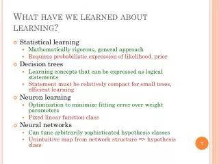
1. What have we learned about learning? • Statistical learning • Mathematically rigorous, general approach • Requires probabilistic expression of likelihood, prior • Decision trees • Learning concepts that can be expressed as logical statements • Statement must be relatively compact for small trees, efficient learning • Neuron learning • Optimization to minimize fitting error over weight parameters • Fixed linear function class • Neural networks • Can tune arbitrarily sophisticated hypothesis classes • Unintuitive map from network structure => hypothesis class

2. Support Vector Machines

3. SVM Intuition • Find “best” linear classifier • Hope to generalize well

4. Linear classifiers • Plane equation: 0 = x1θ1+ x2θ2 + … + xnθn + b • If x1θ1 + x2θ2 + … + xnθn + b > 0, positive example • If x1θ1 + x2θ2 + … + xnθn + b < 0, negative example Separating plane

5. Linear classifiers • Plane equation: 0 = x1θ1+ x2θ2 + … + xnθn + b • If x1θ1 + x2θ2 + … + xnθn + b > 0, positive example • If x1θ1 + x2θ2 + … + xnθn + b < 0, negative example Separating plane (θ1,θ2)

6. Linear classifiers • Plane equation: x1θ1+ x2θ2 + … + xnθn + b = 0 • C = Sign(x1θ1 + x2θ2 + … + xnθn + b) • If C=1, positive example, if C= -1, negative example Separating plane (θ1,θ2) (-bθ1, -bθ2)

7. SVM: Maximum Margin Classification • Find linear classifier that maximizes the margin between positive and negative examples Margin

8. Margin • The farther away from the boundary we are, the more “confident” the classification Margin Not as confident Very confident

9. Geometric Margin • The farther away from the boundary we are, the more “confident” the classification Margin Distance of example to the boundary is its geometric margin

10. Key Insights • The optimal classification boundary is defined by just a few (d+1) points: support vectors • Numerical tricks to make optimization fast Margin

11. Nonseparable Data • Cannot achieve perfect accuracy with noisy data • Regularization parameter: • Tolerate some errors, cost of error determined by some parameter C • Higher C: more support vectors, lower error • Lower C: fewer support vectors, higher error

12. Soft Geometric Margin Regularization parameter minimize Where Errori indicatesa degree of misclassification Errori: nonzero only for misclassified examples

13. Can we do better?

14. Motivation: Feature Mappings • Given attributes x, learn in the space of features f(x) • E.g., parity, FACE(card), RED(card) • Hope CONCEPT is easier to learn in feature space • Goal: • Generate many features in the hopes that some are predictive • But not too many that we overfit (maximum margin helps somewhat against overfitting)

15. VC dimension • In an N dimensional feature space, there exists a perfect linear separator for n <= N+1 non-coplanar examples no matter how they are labeled ? + - + - + - + + - -

16. What features should be used? • Adding linear functions of x’s doesn’t help SVM separate non-separable data • Why? • But it may help improve generalization (particularly, badly-scaled datasets). Why? • But nonlinear functions may help…

17. Example x2 x1

18. Example • Choose f1=x12, f2=x22, f3=2 x1x2 x2 f3 f2 f1 x1

19. Example • Choose f1=x12, f2=x22, f3=2 x1x2 x2 f3 f2 f1 x1

20. Polynomial features • Original features • x1,…,xn • Quadratic features • x12…xn2, x1x2, …, x1xn, … , xn-1xn (n2 features possible) • Linear classifiers in feature space become ellipses, parabolas, and hyperbolas in original space! • [Doesn’t help to add features like 3x12 - 5x1x3. Why?] • Higher order features also possible • Increase maximum power until data is linearly separable? • SVMs implement these and other feature mappings efficiently through the “kernel trick”

21. Results • Decision boundaries in feature space maybe highly curved in original space! • More complex: better fit, more possibility to overfit

22. Overfitting / underfitting

23. Comments • SVMs often have very good performance • E.g., digit classification, face recognition, etc • Still need parametertweaking • Kernel type • Kernel parameters • Regularization weight • Fast optimization for medium datasets (~100k) • Off-the-shelf libraries • libsvm, SVMlight

24. Nonparametric Modeling(memory-based learning)

25. So far, most of our learning techniques represent the target concept as a model with unknown parameters, which are fitted to the training set • Bayes nets • Linear models • Neural networks • Parametric learners have fixed capacity • Can we skip the modeling step?

26. - - + - + - - - - + + + + - - + + + + - - - + + Example: Table lookup • Values of concept f(x) given on training set D = {(xi,f(xi)) for i=1,…,N} Example space X Training set D

27. - - + - + - - - - + + + + - - + + + + - - - + + Example: Table lookup • Values of concept f(x) given on training set D = {(xi,f(xi)) for i=1,…,N} • On a new example x, a nonparametric hypothesis h might return • The cached value of f(x), if x is in D • FALSE otherwise Example space X Training set D A pretty bad learner, because you are unlikely to see the same exact situation twice!

28. Nearest-Neighbors Models • Suppose we have a distance metricd(x,x’) between examples • A nearest-neighbors model classifies a point x by: • Find the closest point xi in the training set • Return the label f(xi) X - + + - + - + - - + Training set D - +

29. Nearest Neighbors • NN extends the classification value at each example to its Voronoi cell • Idea: classification boundary is spatially coherent (we hope) Voronoi diagram in a 2D space

30. Nearest Neighbors Query • Given dataset D = {(x1,f(x1)),…,(xN,f(xN))}, distance metric d • Brute-Force-NN-Query(x,D,d): • For each example xi in D: • Compute di = d(x,xi) • Return the label f(xi) of the minimum di

31. Distance metrics • d(x,x’) measures how “far” two examples are from one another, and must satisfy: • d(x,x) = 0 • d(x,x’) ≥ 0 • d(x,x’) = d(x’,x) • Common metrics • Euclidean distance (if dimensions are in same units) • Manhattan distance (different units) • Axes should be weighted to account for spread • d(x,x’) = αh|height-height’| + αw|weight-weight’| • Some metrics also account for correlation between axes (e.g., Mahalanobis distance)

32. Properties of NN • Let: • N = |D| (size of training set) • d = dimensionality of data • Without noise, performance improves as N grows • k-nearest neighbors helps handle overfitting on noisy data • Consider label of k nearest neighbors, take majority vote • Curse of dimensionality • As d grows, nearest neighbors become pretty far away!

33. Curse of Dimensionality • Suppose X is a hypercube of dimension d, width 1 on all axes • Say an example is “close” to the query point if difference on every axis is < 0.25 • What fraction of X are “close” to the query point? ? ? d=2 d=3 d=10 d=20 0.52 = 0.25 0.53 = 0.125 0.510= 0.00098 0.520= 9.5x10-7

34. Computational Properties of K-NN • Training time is nil • Naïve k-NN: O(N) time to make a prediction • Special data structures can make this faster • k-d trees • Locality sensitive hashing • … but are ultimately worthwhile only when d is small, N is very large, or we are willing to approximate See R&N

35. Aside: Dimensionality Reduction • Many datasets are too high dimensional to do effective supervised learning • E.g. images, audio, surveys • Dimensionality reduction: preprocess data to a find a low # of features automatically

36. Principal component analysis • Finds a few “axes” that explain the major variations in the data • Related techniques: multidimensional scaling, factor analysis, Isomap • Useful for learning, visualization, clustering, etc University of Washington

37. Next time • In a world with a slew of machine learning techniques, feature spaces, training techniques… • How will you: • Prove that a learner performs well? • Compare techniques against each other? • Pick the best technique? • R&N 18.4-5