Download
1 / 15
150 likes | 261 Vues
Assessing Predictions of CME Time-of-Arrival and 1 AU Speed to Observations. Angelos Vourlidas. STEREO Integrates Closely Remote & In-Situ Observations. Lynch et al 2010. P. φ. H-M. Many Methods for Measuring CMEs in 3D!. Direct Reconstruction

E N D
Assessing Predictions of CME Time-of-Arrival and 1 AU Speed to Observations Angelos Vourlidas Vourlidas- SHINE 2012
STEREO Integrates Closely Remote & In-Situ Observations Lynch et al 2010 Vourlidas- SHINE 2012
P φ H-M Many Methods for Measuring CMEs in 3D! • Direct Reconstruction • Forward Modeling (Thernisien et al, Wood et al) • Geometric techniques • Triangulation • Using images (H-t) • Using J-maps (ε- t) (Liu et al 10) • Using masses (Colaninno & Vourlidas 09) • Using polarization (de Koning et al 09) • Point-P (Kahler & Webb ‘07) • Fixed-φ(Sheeley et al. ‚99) • Harmonic Mean (Lugaz et al `09) • Self-similar expansion (Möstl & Davies, 2012) Vourlidas- SHINE 2012
Kinematic Model of the Apr. 26 CME Slide courtesy of B. Wood NOTE: This is a kinematic model for the leading edge of the flux rope component, not the front ahead of it. Vourlidas- SHINE 2012
Speed/ToA depends on fitting method Colaninno thesis (ArXiv)Colaninno & Vourlidas (in prep) • black plus signs - front height from GCS model. • gray bars - estimated measurement error. (COR1 = 1, COR2 = 2, HI1=5, HI2 = 10 Rs). • dotted vertical line - arrival time of CME in situ. • green line - smooth spline fit with linear extrapolation to 1AU using the mean velocity of the last 2 hours of spline fit • green dashed line - spline speed • blue line – 2nd order fit ; dashed line – 2nd order speed • red line – 1st order fit ; dashed line – 1st order speed Vourlidas- SHINE 2012
More examples Vourlidas- SHINE 2012
Comparison of ToA & Speed Predictions to Observations Vourlidas- SHINE 2012
Current state of arrival predictions from Lugaz et al (2010) and Liu et al (2010a,b) From Colaninno PhD Thesis Current Earth-impact accuracy: 6.7 hours Vourlidas- SHINE 2012
Open Issues • Fitting method/function for Height-time curves? • Geometry of CME front and LOS? • Interaction with ambient solar wind. • Rotations, deflections, etc. ToA Error due to Projection Sky plane CME at Earth in projection HI-2 Vourlidas- SHINE 2012
Comparing Imaging to in-situ:ICME Rotations and Deflections Isavnin et al (2012) • In-situ • Imaging CME rotate CW in the inner heliosphere CME deflect towards equator in the inner heliosphere
Imaging CIRs with HI2: The 2008 January 31 CI Study the Evolution of CIRs in 3D Wood et al 2011 HI2-B HI2-A 3D CIR model Synthetic HI2-B image Synthetic HI2-A image Vourlidas- SHINE 2012
Building a 3-D CIR Wood et al 2011 The following equations define the shape of a 2-D CIR shape in cylindrical coordinates in 3-D space, where ψ[0,2π] and η[-1,1]. A 3-D density distribution is then derived by assuming a Gaussian density profile normal to the 2-D CIR shape, such that if (r,,z) is the distance of a point from the CIR midplane, then For our morphological purposes, we simply set nmax=1. For the 2008 January 31 CIR, our best fit has the following parameters: This CIR maps back to a bifurcated streamer near the Sun, which surrounds a coronal hole. = 0.802 AU/rad C = 6.091 rad = 0.7 = 1.48 rad n = 0.0098 AU Vourlidas- SHINE 2012
Visibility of CIRs Sheeley and Rouillard (2010) t1 t1 t2 A t2 B CIRs are best seen from region t2, which from Ahead is further away than from Behind Vourlidas- SHINE 2012
Using SECCHI/HI to predict CIR arrival Davis et al 2012 • ACE: Peak= 10 cm-3, FWHM +31h • SECCHI: Peak= 9.5 cm-3, FWHM +58h BUT • ACE gives warning of 20-60 min. • SECCHI gives warning of (at least) 24h. HI imaging is a better tool than in-situ: • Sees streams several days before Earth arrival. • Situated outside Sun-Earth line (optimal angle > 40 deg). • Reconstruct 3Dproperties and origin. Hence, an L5 mission is the best platform for CIR SWx and Research. Geomagnetic response vs CIR arrival predicted from SECCHI/HI observations. Vourlidas- SHINE 2012