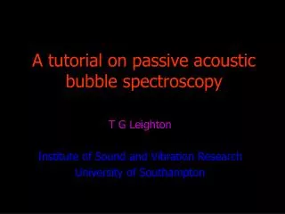
A tutorial on passive acoustic bubble spectroscopy
150 likes | 261 Vues
This tutorial delves into the principles of passive acoustic bubble spectroscopy, highlighting its significance in analyzing bubble dynamics under water. It showcases high-speed photography of raindrops impacting water, accompanied by hydrophone signals that visualize pressure changes over time. The interplay between droplet impacts and bubble generation is illustrated through oscilloscope traces, revealing how bubble size affects sound emission patterns. Understanding these acoustics can lead to quantitative analyses of bubble population distributions, enriching studies in various fields, including oceanography and environmental monitoring.

A tutorial on passive acoustic bubble spectroscopy
E N D
Presentation Transcript
A tutorial on passive acoustic bubble spectroscopy T G Leighton Institute of Sound and Vibration Research University of Southampton
Pressure Time On the screen you see a photograph, taken by Hugh Pumphrey which shows, on the left high speed photography of a raindrop hitting water (the black horizontal line half way through the screen is the air/water interface); and on the right we see an oscilloscope trace of the hydrophone signal, which plots pressure in the horizontal direction and time running down the frame. (f) (a) Air Interface Water Drop (b) (g) (c) (h) The droplet can be seen hitting the water in frame (a). It causes a crater to form up to frame (e) [the black hemisphere visible at the base of frames (b) onwards is the hydrophone]. The crater begins to close, and it is not until frame (g) that the hydrophone shows a signal. This is coincident with a bubble being pinched off from the bottom of the crater. It is the bubble pulsation which causes the exponentially decaying sinusoidcharacteristic of the entrainment, the sound emitted when the bubble is entrained. (d) (i) (e) (j)
raindrop crater bubble In the final frame the closing of the crater produces a jet. In the picture above. In the photograph above we see a clearer picture of a bubble which has just been entrained beneath a closing crater. A second raindrop is coming down onto the water surface. jet
The exponentially decaying sinusoid seen in the hydrophone signal generated when a bubble is “pinched off” is typical of a lightly-damped oscillator, the system which air bubbles in water mimic at low amplitude.
The natural frequency at which the bubble rings is, to an approximation , inversely proportional to the equilibrium bubble radius, R0. Natural frequency ~1/R0
A hydrophone record taken in a babbling brook shows a series of these exponentially decaying sinesoids, which corresponds to the entrainments of about 9 bubbles. The frequency of oscillation gives the bubble size: just like bells of different sizes, big bubbles give out low notes and small bubbles give out high notes. It is therefore apparent that the penultimate bubble (marked C) was smaller than the first bubble (A), and that bubbles B and D were the largest bubbles detected. A B D Natural frequency ~1/R0 C A hydrophone record taken in a babbling brook
The inversion: The ‘inversion’ we would now like to undertake would be to obtain the bubble population size distributions from the acoustic information. In fact, in the last slide we just did this in a qualitative way by comparing the relative natural frequencies of any bubbles we can identify. However we may wish to do this in a quantitative way, when the exponentially decaying sinusoids generated by various bubbles might overlap or be hidden in noise (and so not be as readily identifiable as on the last slide). To do this we need a model of how the bubble generates the sound. That model is a lightly damped harmonic oscillator, because we have seen from the previous slides that the bubbles produce a pressure emission which to first order resembles the exponentially decaying sinusoid that is characteristic of the lightly damped oscillator. To summarise in note form: • Inversion: Obtaining bubble population size distributions from the acoustic information • Need model • Lightly-damped harmonic oscillator
The natural frequency and damping of a bubble, when it is modelled as a lightly damped oscillator, have been available in the literature for many decades (note however that these expressions are valid only for monochromatic free field emissions). Natural frequency (Minnaert, 1933): Damping (Devin, 1959):
The bubble natural frequency (as given by Minnaert in 1933) and the damping (as given by Devin) can be combined in a model which can be used to obtain the bubble size distributions from the natural acoustic emissions. This process is called passive acoustic bubble spectroscopy. It is used for many purposes, including those listed in purple: Passive acoustic bubble spectroscopy • Atmosphere/ocean flux of momentum, energy and mass • Shallow water acoustics • Ambient noise • Communication and sensors • Precipitation • Wave dynamics You may wish to contrast this passive acoustic bubble spectroscopy with active acoustic bubble spectroscopy, the topic of it short tutorial which can be found by clicking here
However one key question is, “how do we know that the results of such an inversion are correct?” Let us undertake an example problem. We ask a computer to construct a time series of the hydrophone signal generated by a known bubble population using the models by Devin and Minnaert (mentioned earlier). We instruct the computer to use an emission amplitude weighting, which shows that for example bigger bubbles give out more sound than smaller bubbles, and bubbles close to the hydrophone contribute to the received signal more sound than those further away. We also ask the computer to add random noise, just as one would find in nature. Once we have told the computer how to construct an artificial hydrophone trace from a known bubble population, we tell it to generate a random population of bubbles: The computer knows what the population is, but we do not. Therefore we can undertake an inversion, estimate the bubble population from the sound signal, and then compare our estimation with the actual bubble population that the computer put in. The steps of this process of summarised on the next slide:
Passive acoustic bubble spectroscopy An example to investigate the question “how do we know result of inversion is correct?” Method: Construct the time series from a known bubble population, using: Minnaert/Devin models Emission amplitude weighting Noise Randomisation
(a) Passive acoustic bubble spectroscopy Frequency (Hz) (b) 50 bubbles/second Time (s) Here is a first example showing (a) the artificially constructed hydrophone signal when fifty bubbles per second are introduced without noise. The spectrogram of this signal is shown in (b). This plots high acoustic energy as ‘hot’ colours, distributed across frequency bands as indicated in the vertical axis, at times as marked on the horizontal axis. In the spectrogram it is easy to identify the frequency of the individual bubbles and their amplitude. You can hear this signal by clicking on the loud speaker, it is very easy to here the individual bubble signals. However it does not sound like realistic rain or a babbling brook.
Passive acoustic bubble spectroscopy A 50 bubbles/second + noise Now we see the result when a hydrophone signal is constructed with the same rate of bubble generation (50 per second), but the computer adds random noise similar to that which would be encountered in nature. The result sounds a little more like rain or a babbling book (click on the loudspeaker). You should be able to clearly here at the high amplitude, low-frequency signal from a large bubble near the beginning of the recording (labelled A).
Passive acoustic bubble spectroscopy A 2500 bubbles/second Now we see the result when a hydrophone signal is constructed, with added noise, but the bubble generation rate has increased to 2500 per second). The result sounds a lot more like rain or a babbling book (click on the loudspeaker). You should be able to clearly here at the high amplitude, low-frequency signal from a large bubble near the end of the recording (labelled A).
When this final time series is inverted, we obtained the bubble population given in (b), the bottom graph (the red curve corresponding to the bubbles which are generated in the first second of the hydrophone trace, and the yellow curve of those generated in the second second). Having in the bottom graph estimated the bubble population the computer used to generate the time series, we can now look at the top graph (a)and see the actual bubble population the computer had in mind. The to match closely indicating that our inversion was successful. 2500 bubbles/second Actual number of bubbles (a) Result of inversion (b)