Introduction to Signal Processing for Acoustic Neutrino Detection
300 likes | 391 Vues
Learn about signal processing techniques for acoustic neutrino detection, including Fourier analysis, SVD, and more. Discover how signal processing enhances accuracy and efficiency in analyzing acoustic data. Explore optimal filter design and classification algorithms. Enhance your understanding of Singular Value Decomposition and its applications in data analysis. Dive into examples of applying signal processing in acoustic sciences and statistical analysis.

Introduction to Signal Processing for Acoustic Neutrino Detection
E N D
Presentation Transcript
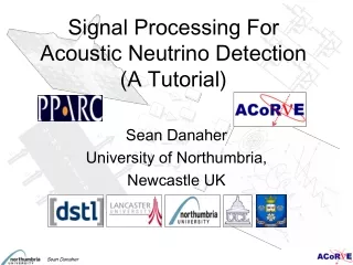
u1 [A] M I M O S Y S T E M u2 -K- 1 y1 z [A] u3 -K- 1 + + z 1 -K- - - z u4 -K- + + y2 - 1 - z -K- 1 z -K- y3 -K- 1 z Signal Processing For Acoustic Neutrino Detection (A Tutorial) Sean Danaher University of Northumbria, Newcastle UK
What is Signal Processing? u1 [A] M I M O S Y S T E M u2 -K- 1 y1 z [A] u3 -K- 1 + + z 1 -K- - - z u4 -K- + + y2 - 1 - z -K- 1 z -K- y3 -K- 1 z • Used to model signals and systems where there is correlation between past and current inputs/outputs (in space or time) • Two broad categories: Continuous and Sampled processes • A host of techniques Fourier, Laplace, State space, Z-Transform, SVD, wavelets…… • Fast, accurate, robust and easy to implement • Sadly also a big area. Engineers spend years learning the subject (Not long Enough!) • Smart as Physicists are I can’t cover a 3+ year syllabus in 40 minutes! • Notation (not just i and j)!
How Can Signal Processing be used in Acoustic Neutrino Detection? u1 [A] M I M O S Y S T E M u2 -K- 1 y1 z [A] u3 -K- 1 + + z 1 -K- - - z u4 -K- + + y2 - 1 - z -K- 1 z -K- y3 -K- 1 z • At Virtually all stages of the process • Accurate Parameterisation of distributions with no amenable analytical form e.g. Shower Energy distribution profiles • Speed up computation e.g. Acoustic integrals by many orders of magnitude • Design, Understand, simulate Hydrophones, Microphones and other acoustic transducers (and amplifiers) • Design, Understand, simulate filters both analogue and digital (tailored amplitude, phase response, minimise computing time) • Estimate and recreate noise and background spectra • Design Optimal Filters e.g. Matched Filters • Design Optimal Classification Algorithms (Separating Neutrino Pulses from Background) • Improve Reconstruction accuracy…………… • Will cover 1-5 in this talk……
Singular Value Decomposition u1 [A] M I M O S Y S T E M ( ( ( ) ) ) u2 -K- 1 y1 z [A] u3 -K- 1 + + z 1 -K- - - z u4 -K- + + y2 - 1 - z -K- 1 WLVT z -K- y3 -K- 1 z Decompose the Data matrix into 3 matrices. When multiplied we get back the original data. W and V are unitary. L contains the contribution from each of the eigenvectors in descending order along main diagonal. We can get an approximation of the original data by setting the L values to zero below a certain threshold Similar techniques are used in statistics CVA, PCA and Factor Analysis Based on Eigenvector Techniques Good SVD algorithms exist in ROOT and MATLAB
SVD II u1 [A] M I M O S Y S T E M u2 -K- 1 y1 z [A] u3 -K- 1 + + z 1 -K- - - z u4 -K- + + y2 - 1 - z -K- 1 z -K- y3 -K- 1 z • Somewhere between vector five and seven we get the “Best” representation of the data • Better than the observation as noise filtered out • Highly compressed (only 1-2% of original size e.g. 6/500x1.5) • Have basis vectors for data so can produce “similar” data+++ SVD done on Noisy data
Building the Radial Distribution u1 [A] M I M O S Y S T E M u2 -K- 1 y1 z [A] u3 -K- 1 + + z 1 -K- - - z u4 -K- + + y2 - 1 - z -K- 1 z -K- y3 -K- 1 z 4 examples chosen have maximum variation in shape Hadronic Component using Geant IV • SVD works well with the radial distribution • Three vectors sufficient to fit the data • Can use a linear mixture of these three vectors as input to the Acoustic MC We Reproduce both the shape and variation
Acoustic Integrals Slow decay fast thermal energy deposition • Band limited by • Water Properties • Attenuation
Method I 4 u1 x 10 0.1 0.5 3 0.05 2 -0.2 0 Pressure (Pa) 0 P (arbitrary) [A] 0 0.2 M I M O S Y S T E M -0.05 3 -0.1 2.5 -6 -4 -2 0 2 4 6 -0.5 -5 0 5 -4 Time (s) u2 Time (ps) x 10 -K- 4 1 5 2 y1 z [A] u3 -K- 6 Radial Distribution 1 + + 7 1.5 z Frequency 1 -K- - - z u4 8 -K- + + y2 - 1 - 1 9 z -K- 1 10 z -K- 0.5 11 y3 -K- 12 1 0 z 0 2 4 6 8 10 12 Longitudinal Distance (m) • Throw a number if MC points ~107 • Assume the energy at each point in the cascade deposited as a Gaussian Distribution. • Calculate distance to observer from each point • Propagate the Gaussian to the observer (an analytical solution is known for this) • Sum over all the points • Provided the width of the Gaussian is small in comparison to the shower radius we will get the pressure pulse Expensive 5 flops per time point If using 1024 points on time axis 5*1024*1e7=5.1e10 flops Need to do this thousands of times for different distances, angles, distributions, etc.
The Convolution Integral u1 M I M O S Y S T E M u2 y1 u3 + + - - u4 + + y2 - - y(t) Electrical Pulse s(t) Bipolar Acoustic Pulse h(t) Impulse response high pass filter (SAUND) y3 Given a signal s(t) and a system with an impulse response h(t) (response to (t)) then y(t) to an arbitrary input is given by We can use this to process all the MC points in the cascade simultaneously
A Few examples u1 [A] M I M O S Y S T E M u2 -K- 1 y1 z [A] u3 -K- 1 + + z 1 -K- - - z u4 -K- + + y2 - 1 - z -K- 1 z -K- y3 -K- 1 z RC circuit Mixed signal This situation is similar to our acoustic integral * = 2d
Convolution Theorem u1 [A] M I M O S Y S T E M u2 -K- 1 y1 z [A] u3 -K- 1 + + z 1 -K- - - z u4 -K- + + y2 - 1 - z -K- 1 z -K- y3 -K- 1 z Convolution in the time domain is Multiplication in the frequency domain (and visa versa) • Will speed the process still further • Convolution very expensive computationally (o=n2) • Convert the signal and impulse response to the frequency domain (Fourier Transform) • Provided the number of points n=2mveryefficient FFTs o=n log n • Multiply and take Inverse Transform
Acoustic Integrals II u1 [A] M I M O S Y S T E M u2 -K- 1 y1 z [A] u3 -K- 1 + + z 1 -K- - - z u4 -K- y2 + + 1 - - z -K- 1 z -K- y3 -K- 1 z • Assume each point produces a Delta Function • The sampled equivalent of a Delta function is 1 • The integral can be done using a histogram function • (modern histogram algorithms are very efficient) • The derivative can be done in the frequency domain (d/dt i No overhead) • We then convolve the response with the entire signal
Only Histogram depends on the number of MC points u1 [A] M I M O S Y S T E M u2 -K- 1 y1 z [A] u3 -K- 1 + + z 1 -K- - - z u4 -K- + + y2 - 1 - z -K- 1 z -K- y3 -K- 1 z Derivative j FT of Exyz Water Attenuation Blackman window Histogram: 103 flops Scale histogram by 1/d: 103 flops (only needed in near field) FFT nLogn c 104 flops Multiplication c 4x10³ flops IFFT nLogn c 104 flops 6 orders of magnitude less than approach 1 Limitation: Will not work if volume of the integral is so great that attenuation varies significantly (Large 100+m source in near field)
State Space Analysis u1 M I M O S Y S T E M u2 y1 u3 u4 y2 y3 MIMO systems Mixed Mechanical/electrical models etc Matrix Based Method Mode 1 Quantum Mechanics Mode 14 All modern control algorithms use SS methods. Mode 100 Pictured 20000 state simulation of a square acoustic membrane: (100x100 masses 2 states x and v) A Matrix 400x106 elements
SS Implementation u1 M I M O S Y S T E M u2 y1 u3 u4 y2 y3 States Inputs • States are degrees of freedom of the system. Things that store energy • Capacitor Voltages • Inductor currents • Positions and Velocities of masses A B States D Outputs C A is of size States States B is of size States Inputs C is of size Outputs States D is of size Outputs Inputs
Simple Example LC u1 M I M O S Y S T E M u2 y1 u3 Response to Initial Conditions 1.5 u4 1 y2 0.5 Voltage 0 -0.5 -1 Amplitude -1.5 1.5 1 y3 0.5 Current 0 -0.5 -1 -1.5 0 5 10 15 20 25 30 35 40 Time (sec) Maths simple to implement Example shows the behaviour with an initial 1V on the Capacitor (1F) and 1A flowing through the inductor (1H)
Speaker/Microphone u1 [A] M I M O S Y S T E M u2 -K- 1 Mechanically Force produced by current y1 z [A] u3 -K- Loss to air term 1 + + z 1 -K- - - z u4 N -K- + + S y2 Bode Diagram - 1 - -60 z -80 -K- 1 -100 z Magnitude (dB) -120 -K- -140 -160 y3 90 -K- 1 0 Phase (deg) z -90 -180 2 3 4 5 6 10 10 10 10 10 Frequency (rad/sec) Frame Cone Magnet assembly Magnet assembly Coil x1=x, (position) x2=dx/dt, (velocity) x3=i, (current) Electrically coil moving in a magnetic field Creates an EMF Step Response -4 x 10 2.5 2 1.5 Amplitude 1 0.5 0 -0.5 0 0.5 1 1.5 2 2.5 3 Time (ms)
Simple Hydrophone Model u1 [A] M I M O S Y S T E M u2 -K- 1 y1 z [A] u3 -K- 1 + + z 1 -K- - - z u4 -K- + + y2 - 1 - z -K- 1 Simulated Hydrophone signal z 25 -K- 20 15 y3 10 -K- Amplitude (Arbitrary) 5 1 0 z -5 -10 -15 25 30 35 40 45 50 Time (eq. cm) Heart of Hydrophone Piezo electric crystal Piezo electric effect Omni works in breathing mode 40cm 30cm = 0.09 =5e-3 “Erlangener” water tank (Niess) 3rd order simulation. Do we need higher? Gaussian cross-section
Acoustic Simulation u1 M I M O S Y S T E M u2 y1 u3 u4 y2 y3 • Bipolar Pulse • 1000 element simulation • Two types of medium; Heavy and light • pulse reflects against walls • mismatch between sections • velocity on each section • amplitude change • dispersion Enhance to 2D? Embed Hydrophone models etc.?
Butterworth Filter + + + + - - - - 1930s Stable Good Frequency Response • Note Impulse response • Output Delay • Oscillation
Implementation Passive Filters 1st Order Familiar RC 2nd Order LRC = 3rd Order “” + + + + - - - - = + + - - At acoustic frequencies easiest to use op-amps. Expensive to make high precision lossless inductors Cascade 2nd Order sections to make Butterworth high order filters Ra Rb
Recovering Phase information + + + + - - - - e.g. SAUND Data It is trivial to design digital filters which have a constant group delay d/dand hence no phase distortion 0.15 S+N causal non causal 0.1 0.05 Amplitude (Arbitrary) 0 If however we know the filter response e.g. Butterworth we can run the data through the filter backwards. -0.05 -0.1 0 0.2 0.4 0.6 0.8 1 1.2 time (s) -3 x 10 This increases the order of the filter by a factor of 2
The Digital Filter [A] -K- 1 z [A] -K- 1 z 1 -K- z 6 6 8 14 9 23 7 30 2 32 4 36 9 45 9 54 4 58 9 67 Perfect Integrator -K- 1 z -K- 1 Called IIR or AR z -K- -K- 1 z The digital filter is simple! Based upon sampled sequences Negative coefficients =>Causal Simple moving average Filter 10 5 2 6 6 4 5 5.5 9 7 8 8.5 5 6.5 0 2.5 8 4 4 6 Crude low-pass Called FIR or MA
The Z Transform and Sampled Signals [A] -K- 1 z [A] -K- 1 z 1 -K- z -K- 1 Geometric sequences are of prime interest because z -K- 1 z -K- is a geometric sequence -K- 1 z
A few z transforms [A] 1 3 2 0 1 -K- 0 -1 -1 -2 1 -3 -1 0 1 z -4 [A] 0 5 10 15 20 25 30 -K- 1 1 10 z 0 1 -K- 5 0 z -K- -1 -5 -10 1 -15 z -K- 0 5 10 15 20 25 30 1 1 z Frequency Response -K- 20 2 0 1.5 15 1 -K- -1 0.5 1 10 0 z -0.5 5 -1 -1.5 0 5 10 15 20 25 30 0 0 0.2 0.4 0.6 0.8 1 Fraction of Nyquist frequency Poles must be inside the unit circle for stability
Simple Transfer Function [A] 3 -K- 2.5 2 1 )| w 1.5 z |H( [A] -K- 1 1 0.5 z 1 -K- 0 0 0.2 0.4 0.6 0.8 1 z frequency (Nyquist=1) -K- 60 1 50 z -K- 1 40 z 30 -K- 1 20 10 -K- 0 1 0 0 0.2 0.4 0.6 0.8 1 frequency (Nyquist=1) z -1 Frequency response simply determined by running around the unit circle Corresponds to the Nyquist Frequency (fs/2) ) (degrees) w H( Ð
Notch Filter [A] Fs=1000Hz 1.4 -K- 1.2 1 z [A] 1 -K- 1 1 0.8 )| z 1 -K- w /5 0 |H( z 0.6 -K- -1 1 1.5 0.4 z -1 0 1 -K- 1 1 z -K- 0.5 0.2 0 -K- 0 -0.5 0 100 200 300 400 500 1 frequency -1 z -1.5 0 0.05 0.1 0.15 0.2 0.25 Time Signal buried in 100Hz Recovered signal
4 3 2 Spectral Analysis First 500 of 2048 data points 1 [A] -K- 1 z [A] Autocorrelation 1 -K- 0 Amplitude 1 0.5 z Amplitude (relative) 1 -K- 0 z -K- 0.18 fft -0.5 -150 -100 -50 0 50 100 150 ac 1 0.16 Lag lpc z -K- 0.14 1 -1 z 0.12 -K- 0.1 Amplitude(Relative) 0.08 -K- 0.06 1 0.04 z 0.02 0 0 0.2 0.4 0.6 0.8 1 -2 Frequency (relative) -3 -4 0 100 200 300 400 500 Sample number • Using the Fourier Transform is seldom the best way to get a spectrum. Normally methods based around • Autocorrelation (AC) • Linear Prediction are used AC method Use FT of AC To get PSD Linear Prediction All pole filter driven by white noise. Need to choose the order with care. But can now reproduce the spectrum
Spectral estimation example [A] pitch voiced/unvoiced -K- switch vocal tract 1 synthesized gain filter speech z [A] -K- noise 1 z 1 -K- z spectrum of frame 48 Impulse Response -K- 8 2 7 1 1.5 6 z -K- 1 1 5 z |h()| h(t) 4 0.5 -K- 3 0 2 -0.5 -K- 1 1 0 -1 0 1000 2000 3000 4000 0 10 20 30 40 50 z Sample [n] • 8 bit 8kHz • Split speech into frame 240 samples long • Use LPC10 to estimate spectrum • Reconstruct 64k 2.4k 933 Frequency (Hz)
Conclusions u1 [A] M I M O S Y S T E M u2 -K- 1 y1 z [A] u3 -K- 1 + + z 1 -K- - - z u4 -K- + + y2 - 1 - z -K- 1 z -K- y3 -K- 1 z • SP Techniques Useful • Thanks for listening • Questions