Understanding Correlation: Pearson, Spearman, and Kendall Methods Explained
This guide explores the concept of correlation, primarily focusing on Pearson's r, Spearman's rho, and Kendall's tau. It explains how these statistical measures assess relationships between variables. Pearson's r indicates the strength of linear relationships, with values ranging from -1 to +1, while Spearman's rho and Kendall's tau are suitable for ordinal data. We also touch on nominal measures like Cramer's V and odds ratios. Additionally, we provide practical examples using R code for computing these correlations and their significance, aiding in data analysis.

Understanding Correlation: Pearson, Spearman, and Kendall Methods Explained
E N D
Presentation Transcript
Association Predicting One Variable from Another
Correlation • Usually refers to Pearson’s r computed on two interval/ratio scale variables. • It measures the degree to which variance in one variable is “explained” by a second variable • It measures the strength of a linear relationship between the variables
Properties of r • r is symmetrical and varies from -1 to +1 • 0 indicates no correlation or relationship • ±1 indicates a perfect correlation (knowledge of one variable makes it possible to predict the second one without any error).
Properties of r2 • r2 is symmetrical and varies from 0 to 1 • r2 is the proportion of the variability in one variable that is “explained by” the other variable • cor.test(x, y, method=“pearson”) • cor(x, y, method=“pearson”)
Spearman’s rho • For rank/ordinal data. • Pearson correlation computed on ranks • If Spearman coefficient is larger than Pearson, it may indicate a non-linear relationship • Ties make it difficult to compute p values
Kendall’s tau • For rank/ordinal data • Evaluate pairs of observations (xi, yi) and (xj, yj) • Concordant – (xi > xj) and (yi > yj) OR (xi < xj) and (yi < yj) • Discordant – (xi > xj) and (yi < yj) OR (xi < xj) and (yi > yj)
Kendall’s tau b • Divide by total number of pairs adjusted for all ties
Kendall’s tau c • For grouped (tabled data) where the table is not square (rows ≠ columns)
Nominal Measures • Measures based on Chi-Square: • Phi coefficient • Cramer’s V • Contingency coefficient • Odds ratio
Phi and Cramer’s V • Phi ranges from 0 to 1 in a 2x2 table but can exceed 1 in larger tables. Cramer’s V adds a correction to keep the maximum value at 1 or less:
Contingency Coefficient • Ranges from 0 to <1 depending on the number of rows and columns with 1 indicating a high relationship and 0 indicating no relationship
Odds Ratio • For 2 x 2 tables it shows the relative odds between the two variables
> Table <- xtabs(~Sex+Goods, data=EWG2) > Table Goods Sex Absent Present Female 38 28 Male 16 30 > ChiSq <- chisq.test(Table) > ChiSq Pearson's Chi-squared test with Yates' continuity correction data: Table X-squared = 4.7644, df = 1, p-value = 0.02905
library(vcd) > assocstats(Table) X^2 df P(> X^2) Likelihood Ratio 5.7073 1 0.016894 Pearson 5.6404 1 0.017552 Phi-Coefficient : 0.224 Contingency Coeff.: 0.219 Cramer's V : 0.224 > cor(as.numeric(EWG2$Sex), as.numeric(EWG2$Goods), use="complete.obs") [1] 0.2244111 > oddsratio(Table, log=FALSE) [1] 2.544643