Boundary Setup Exercise: Radiation

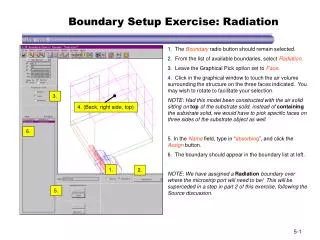
1. Boundary Setup Exercise: Radiation 1. The Boundaryradio button should remain selected. 2. From the list of available boundaries, select Radiation. 3. Leave the Graphical Pick option set to Face. 4. Click in the graphical window to touch the air volume surrounding the structure on the three faces indicated. You may wish to rotate to facilitate your selection. NOTE: Had this model been constructed with the air solid sitting on top of the substrate solid, instead of containing the substrate solid, we would have to pick specific faces on three sides of the substrate object as well. 5. In the Name field, type in “absorbing”, and click the Assign button. 6. The boundary should appear in the boundary list at left. NOTE: We have assigned a Radiation boundary over where the microstrip port will need to be! This will be superceded in a step in part 2 of this exercise, following the Source discussion. 3. 4. (Back, right side, top) 6. 1. 2. 5.

2. 4. Boundary Setup Exercise: Ground Plane 1. The Boundaryradio button should remain selected. 2. From the list of available boundaries, select Perfect E. 3. Leave the Graphical Pick option set to Face. 4. Either rotate the model view to bring the lower face to the front, and click on it, or click as though touching the lower face of the air volume and use the “N” key to shift focus deeper to the lower surface of the air volume and substrate. 5. In the Name field, type in “ground_plane”, and click the Assign button. 6. The boundary should appear in the boundary list at left. NOTE: Since this is being assigned a Perfect E boundary, we could have allowed the automatic “outer” boundary to take care of this face if we wished. 3. 6. 1. 2. 5.

3. 4. 4. 4. Boundary Setup Exercise: Symmetry Plane 1. The Boundaryradio button should remain selected. 2. From the list of available boundaries, select Symmetry. 3. Leave the Graphical Pick option set to Face. 4. Click on the face of the model which bisects the microstrip trace and coax. Once a face is selected, the options for the Symmetry boundary appear below the graphical view. Click again in the model to select the cut faces of the ‘thru_hole_in_wall’ and “coax_outer” cylinders as well. (You may wish to zoom in to assure you have the correct faces selected.) NOTE: Again, if we had defined our air volume to sit atop rather than to contain the substrate, we would need to select the substrate face too. 5. In the parameter space for the boundary, click the radio button for Perfect H type symmetry (E-fields tangential to surface). 6. In the Name field, type in “mag_symmetry”, and click the Assign button. 7. The boundary should appear in the list at left. THIS CONCLUDES PART 1 OF THE BOUNDARY SETUP EXERCISE. DO NOT EXIT THE BOUNDARY/ SOURCE MANAGER. 3. 7. 1. 2. 6. 5.

4. HFSS Ports: A Detailed Look • The Port Solution provides the excitation for the 3D FEM Analysis. Therefore, knowing how to properly define and create a port is paramount to obtaining an accurate analysis. • Incorrect Port Assignments can cause errors due to... • ...Excitation of the wrong mode structure • ...Bisection by conductive boundary • ...Unconsidered additional propagating modes • ...Improper Port Impedance • ...Improper Propagation Constants • ...Differing phase references at multiple ports • ...Insufficient spacing for attenuation of modes in cutoff • ...Inability to converge scattering behavior because too many modes are requested • Since Port Assignment is so important, the following slides will go into further detail regarding their creation.

5. HFSS Ports: Setup Interface Name Field Ports are always named “portN”. Box also includes Assign, Clear, and Options buttons. Lumped Gap Source Port Option Activating enables Port Impedance entry fields. Impedance and Calibration Line Fields ‘Edit Line’ dropdown allows setting, clearing, and relating Imped. and Calib. lines. Mode Entry Field Set port mode solution requirements. Set polarization. Shows impedance and calibration definitions applied, if any. Impedance Multiplier Field Use if symmetry planes intersect ports.

6. HFSS Port Selection: Standard or Gap Source? • When would you choose to use a Gap SourcePort over a Standard Port? • When the model has tightly-spaced lines • When ‘backing’ the port would be too disruptive of internal fields • When a port reference location is difficult to determine using a Standard port • When you’d like to use a voltage gap, but want S-parameter output Gap Source Ports (blue)

7. HFSS Ports: Sizing • A port is an aperture through which a guided-wave mode of some kind propagates • For transmission line structures entirely enclosed in metal, port size is merely the waveguide interior carrying the guided fields • Rectangular, Circular, Elliptical, Ridged, Double-Ridged Waveguide • Coaxial cable, coaxial waveguide, square-ax, Enclosed microstrip or suspended stripline • For unbalanced or non-enclosed lines, however, field propagation in the air around the structure must also be included • Parallel Wires or Strips • Stripline, Microstrip, Suspended Stripline • Slotline, Coplanar Waveguide, etc. A Coaxial Port Assignment A Microstrip Port Assignment (includes air above substrate)

8. HFSS Ports: Sizing, cont. • The port solver only understands conductive boundaries on its borders • Electric conductors may be finite or perfect (including Perfect E symmetry) • Perfect H symmetry also understood • Radiation boundaries around the periphery of the port do not alter the port edge termination!! • Result: Moving the port edges too close to the circuitry for open waveguide structures (microstrip, stripline, CPW, etc.) will allow coupling from the trace circuitry to the port walls! • This causes an incorrect modal solution, which will suffer an immediate discontinuity as the energy is injected past the port into the model volume Port too narrow (fields couple to side walls) Port too Short (fields couple to top wall)

9. 10w, w  h or 5w (3h to 4h), w < h 6h to 10h w h HFSS Ports: Sizing Handbook I • Microstrip Port Sizing Guidelines • Assume width of microstrip trace is w • Assume height of substrate dielectric is h • Port Height Guidelines • Between 6h and 10h • Tend towards upper limit as dielectric constant drops and more fields exist in air rather than substrate • Bottom edge of port coplanar with the upper face of ground plane • (If real structure is enclosed lower than this guideline, model the real structure!) • Port Width Guidelines • 10w, for microstrip profiles with w  h • 5w, or on the order of 3h to 4h, for microstrip profiles with w < h Note: Port sizing guidelines are not inviolable rules true in all cases. For example, if meeting the height and width requirements outlined result in a rectangular aperture bigger than /2 on one dimension, the substrate and trace may be ignored in favor of a waveguide mode. When in doubt, build a simple ports-only model and test.

10. 8w, w  h or 5w (3h to 4h), w < h w h HFSS Ports: Sizing Handbook II • Stripline Port Sizing Guidelines • Assume width of stripline trace is w • Assume height of substrate dielectric is h • Port Height Guidelines • Extend from upper to lower groundplane, h • Port Width Guidelines • 8w, for microstrip profiles with w  h • 5w, or on the order of 3h to 4h, for microstrip profiles with w < h • Boundary Note: Can also make side walls of port Perfect H boundaries

11. HFSS Ports: Sizing Handbook III • Slotline Port Guidelines • Assume slot width is g • Assume dielectric height is h • Port Height: • Should be at least 4h, or 4g (larger) • Remember to include air below the substrate as well as above! • If ground plane is present, port should terminate at ground plane • Port Width: • Should contain at least 3g to either side of slot, or 7g total minimum • Port boundary must intersect both side ground planes, or they will ‘float’ and become signal conductors relative to outline ‘ground’ Approx 7g minimum Larger of 4h or 4g g h

12. HFSS Ports: Sizing Handbook IV • CPW Port Guidelines • Assume slot width is g • Assume dielectric height is h • Assume center strip width is s • Port Height: • Should be at least 4h, or 4g (larger) • Remember to include air below the substrate as well as above! • If ground plane is present, port should terminate at ground plane • Port Width: • Should contain 3-5g or 3-5s of the side grounds, whichever is larger • Total about 10g or 10s • Port outline must intersect side grounds, or they will ‘float’ and become additional signal conductors along with the center strip. Larger of approx. 10g or 10s Larger of 4h or 4g s h g

13. HFSS Ports: Sizing Handbook V; Gap Source Ports Perfect E • Gap Source ports behave differently from Standard Ports • Any port edge not in contact with metal structure oranother port assumed to be a Perfect H conductor • Gap Source Port Sizing (microstrip example): • “Strip-like”: [RECOMMENDED] No larger than necessary to connect the trace width to the ground • “Wave-like”: No larger than 4 times the strip width and 3 times the substrate height • The Perfect H walls allow size to be smaller than a standard port would be • However, in most cases the strip-like application should be as or more accurate • Further details regarding Gap Source Port sizing available as a separate presentation Perfect H Perfect H Perfect E Perfect H Perfect H Perfect H Perfect E

14. HFSS Ports: Spacing from Discontinuities • Structure interior to the modeled volume may create and reflect non-propagating modes • These modes attenuate rapidly as they travel along the transmission line • If the port is spaced too close to a discontinuity causing this effect, the improper solution will be obtained • A port is a ‘matched load’ as seen from the model, but only for the modes it has been designed to handle • Therefore, unsolved modes incident upon it are reflected back into the model, altering the field solution • Remedy: Space your port far enough from discontinuities to prevent non-propagating mode incidence • Spacing should be on order of port size, not wavelength dependent Port Extension

15. HFSS Ports: Single-Direction Propagation Port on Exterior Face of Model • Standard ports must be defined so that only one face can radiate energy into the model • Gap Source Ports have no such restriction • Position Standard Ports on the exterior of the geometry (one face on background) or provide a port cap. • Capshould be the same dimensions as the port aperture, be a 3D solid object, and be defined as a perfect conductor in the Material Setup module Port Inside Modeled Air Volume; Back side covered with Solid Cap

16. HFSS Ports: Mode Count • Ports should solve for all propagating modes • Ignoring a mode which does propagate will result in incorrect S-parameters, by neglecting mode-to-mode conversion which could occur at discontinuities • However, requesting too many modes in the full solution also negatively impacts analysis • Modes in cutoff are more difficult to calculate; S-parameters for interactions between propagating and non-propagating modes may not converge well • What if I don’t know how many modes exist? • Build a simple model of a transmission line only, or run your model in “Ports Only” mode, and check! • You can alter the mode count before running the full solution. • Degenerate mode ordering is controlled with calibration lines (see next slide) Circular waveguide, showing two orthogonal TE11 modes and TM01 mode (radial with Z-component). Neglecting the TM01 mode from your solution would cause incorrect results.

17. HFSS Ports: Degenerate Modes • Degenerate modes have identical impedance, propagation constants • Port solver will arbitrarily pick one of them to be ‘mode(n)’ and the other to be ‘mode(n+1)’ • Thus, mode-to-mode S-parameters may be referenced incorrectly • To enforce numbering, use a calibration line and polarize the first mode to the line • OR, introduce a dielectric change to slightly perturb the mode solution and separate the degenerate modes • Example: A dielectric bar only slightly higher in permittivity than the surrounding medium will concentrate the E-fields between parallel wires, forcing the differential mode to be dominant • If dielectric change is very small (approx. 0.001 or less), impedance impact of perturbation is negligible In circular or square waveguide, use the calibration line to force (polarize) the mode numbering of the two degenerate TE11 modes. This is also useful because without a polarization orientation, the two modes may be rotated to an arbitrary angle inside circular WG. For parallel lines, a virtual object between them aids mode ordering. Note virtual object need not extend entire length of line to help at port.

18. HFSS Ports: Phase Calibration • A second purpose of the calibration line is to control the port phase references • The 2D port eigensolver finds propagating modes on each port independently • The zero degree phase reference is chosen at a point of maximum E-field intensity on the port face. • This occurs twice, with 180 degrees separation, for each 360 degree cycle • Therefore the possibility exists for the software to select inconsistent phase references from port to port, resulting in S-parameter errors • All port-to-port S-parameter phases, e.g. S21, will be off by 180 degrees • Solution: The calibration line defines the preferred direction for the zero degree reference on each port. Which of the above field orientations is the zero degree phase reference? Calibration Line defines...

19. HFSS Ports: Impedance Definitions • HFSS provides port characteristic impedances calculated using the power-current definition (Zpi) • Incident power is known excitation quantity • Port solver integrates H-field around port boundary to calculate current flow • For many transmission line types, the power-voltage or voltage-current definition is preferred • Slot line, CPW: Zpv preferred • TEM lines: Zvi preferred • HFSS can provide these characteristic impedance values, as long as an impedance line is identified • The impedance line defines the line along which the E-field is integrated to obtain a voltage • Often it can be identical to the calibration line For a Coax, the impedance line extends radially from the center to outer conductor (or vice versa). Integrating the E-field along the radius of the coaxial dielectric provides the voltage difference. In many instances, the impedance and calibration lines are the same!

20. HFSS Ports: Impedance Multiplier • When symmetry is used in a model, the automatic Zpi and impedance line-dependant Zpv and Zvi calculations will be incorrect, since the entire port aperture is not represented. • Split the model with a Perfect E symmetry case, and the impedance is halved. • Split the model with a Perfect H symmetry case, and the impedance is doubled. • The port impedance multiplier is just a renormalizing factor, used to obtain the correct impedance results regardless of the symmetry case used. • The impedance multiplier is applied to all ports, and is set during the assignment of any port in the model. Whole Rectangular WG (No Symmetry) Impedance Mult = 1.0 Half Rectangular WG (Perfect E Symmetry) Impedance Mult = 2.0 Half Rectangular WG (Perfect H Symmetry) Impedance Mult = 0.5 ...and for Quarter Rectangular WG? (Both Perfect E and H Symmetry) Impedance Mult. = 1.0

21. Source Setup Exercise: Part 2 • We will now complete the Setup Boundaries/ Sources exercise already begun, by adding the two necessary Ports to the problem • Ports will use both calibration and impedance lines, but will require only one mode on each terminal

22. Source Setup Exercise: Coaxial Port 1. Select the Source radio button. 2. The source list should set by default to Port. 3. Zoom in on your model, or otherwise orient it so you have clear visual access to the extended face of the coaxial line. Click on the face to select it. The port parameter entry fields will now appear. 4. Leave the port name as “port1”, and the number of modes as “1”. 5. Check the box for Use Impedance Line. This enables the Edit Line dropdown menu beside it. In the Edit Line dropdown, pick Set... 6. The side window will prompt you to Set Impedance Start. Define a starting point for the impedance line by clicking in the graphical window to snap to the vertex on the inner conductor, at the topmost point where it intersects the symmetry plane. (A first click may be necessary to activate the window before selecting vertices.) 7. Click the Enter button in the side window to confirm your point selection. The window now shifts to request the vector information. (proceed to next page) 6. 3. 7. 2. 1. 4. 5.

23. 8. Source Setup Exercise: Coaxial Port, cont. The interface will now show a vector from the starting point you defined to the origin. (This is merely a default ‘guess’ at the intended endpoint.) The side window shows vector entry fields. 8. In the graphical window, snap to the point radial from the starting point (on the outer conductor radius, at the topmost intersection with the symmetry plane). The vector fields should update to reflect a Z-directed vector. 9. Press the Enter button on the side window to confirm the vector end point. The side window interface closes, and the completed impedance line is displayed as a red vector with the letter “I”. 10. Check the box for Use Calibration Line. In the enabled Edit Line dropdown to the right, pick Copy Impedance. The vector will now update to include a “C” indication. 11. Press the Assign button to complete the port creation. The boundary list will now update to show “port1” 9. 11. 10.

24. Source Setup Exercise: Microstrip Port Rotate and resize the graphical window so that you have visual access to the microstrip termination end of the model. 1. Source radio button and Port type are already selected. 2. Click on the 2D rectangle provided for the microstrip port face. If the entire face of the air volume is selected, use the Next Behind menu pick or “N” hotkey to shift the selection. 3. Leave the port name as “port2”, and the number of modes as “1”. 4. Use Impedance Line should remain checked from the prior port assignment. In the Edit Line dropdown, pick Set... 5. The side window will prompt you to Set Impedance Start. Define a starting point for the impedance line by clicking in the graphical window to snap to the vertex on the trace, at the point where it intersects the symmetry plane. 6. Click the Enter button in the side window to confirm your point selection. The window now shifts to request the vector information. (proceed to next page) 2. 5. 6. 1. 3. 4.

25. 7. Source Setup Exercise: Microstrip Port, cont. The interface will now show a vector from the starting point you defined to the prior port’s ending point. The side window shows vector entry fields. 7. In the graphical window, snap to the point where the ground plane intersects the symmetry face. 8. Press the Enter button on the side window to confirm the end point. The side window interface closes, and the completed line is displayed. 9. Use Calibration Line should already be checked. In the enabled Edit Line dropdown to the right, pick Copy Impedance. 10. Before assigning the port, we need to set the Impedance Multiplier for the model. Enter a value of 0.5. 11. Press the Assign button to complete the port assignment. You will receive an overlap warning, because the port overlays the earlier “radiation” boundary. After the overlap warning message is dismissed “port2” will show in the boundary list. 12. We are now done with boundary assignment. To verify our assignment, pick Boundary Display from the Model menu. 12. 8. 11. 9. 10.

26. Source Setup Exercise: Verifying Boundaries HFSS will now perform only the initial meshing necessary to subdivide the problem into tetrahedra, so that actual boundary application to the finite element mesh can be viewed. 13. The list of assigned boundaries is on the left. Note that it contains both boundaries we created, plus the boundaries “i_pinn” and “outer”. The “i_pinn” boundaries were assigned as a result of assigning a finite conductivity metal -- copper -- to the pin objects. The “outer” boundary is applied to any surface of the model we did not otherwise define. Highlight “outer” in the boundary listing. 14. Press the Toggle Displaybutton. The mesh on the selected boundary is displayed, indicating the surfaces on which this boundary is applied. Note that it provides the Perfect E definition on the outer conductor of the coax, on the outer conductor of the thru hole, and on the front face of the model which represents the metal module wall. 15. If you wish you may continue displaying additional boundaries. When you are through, press the Close button to return to the Setup Boundaries window. There, pick Exit from the File menu and save when prompted. (The overlap warning will repeat on exit.) 13. 14. 15.