LABOR MARKET EQUILIBRIUM

1. LABOR MARKET EQUILIBRIUM Hewi-Lin Chuang, Ph.D. 2010/03/25

2. 98-101年促進就業方案 • 方案目標： • 促進勞動市場增加就業機會，減少失業問題，以協助降低失業率，於101年達到3.0%之目標。 • 重點工作項目： • 本方案定位為一補強的政策措施，協助降低失業率，涵蓋短、中、長期的作法。 • 規劃主軸之六大策略：「擴大產學合作」、「強化訓練以促進就業與預防失業」、「提升就業媒合成功率減少摩擦性失業」、「提供工資補貼增加就業機會」、「協助創業與自僱工作者」，以及「加強短期促進就業措施」等。 資料來源： http://www.cepd.gov.tw/m1.aspx?sNo=0010829&ex=1&ic=0000015

3. 就業市場指標 資料來源：行政院主計處，中華民國台灣地區人力資源調查統計年報、速報。

4. 失業規模指標 資料來源：行政院主計處，中華民國台灣地區人力資源調查統計年報、速報。

5. Introduction • Labor market equilibrium coordinates the desires of firms and workers, determining the wage and employment observed in the labor market. • Market types: • Perfect Competition • Monopsony: one buyer of labor • Monopoly: one seller of labor • These market structures generate unique labor market equilibria.

6. LABOR MARKET EQUILIBRIUM • Workers prefer to work when the wage is high, and firms prefer to hire when the wage is low. Labor market equilibrium “balance out” the conflicting desires of workers and firms and determines the wage and employment observed in the labor market.

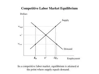
7. 1. Equilibrium in a Single Competitive Labor Market The supply curve gives the total number of employee-hours that agents in the economy allocate to the market at any given wage level; the demand curve gives the total number of employee-hours that firms in the market demand at that wage. Equilibrium occurs when supply equals demand, generating the competitive wage w * and employment E *. Dollars S W* D E* Employment Equilibrium in a Competitive Labor Market Note: There is no unemployment in a competitive labor market. Persons who are not working are also not looking for work at the going wage.

8. Note: The “single wage” property of competitive equilibrium has important implications for economic performance. That is, workers of given skills have the same value of marginal product of labor in all markets. The allocation of workers to firms which equates the value of marginal product across markets is also the allocation which maximizes national income. This type of allocation is called an efficient allocation.

9. (Pareto) Efficiency • Pareto efficiency exists when all possible gains from trade have been exhausted. • When the state of the world is Pareto Efficient, to improve one person’s welfare necessarily requires decreasing another person’s welfare. • In policy applications, ask whether a change can make any one better off without harming anyone else. If the answer is yes, then the proposed change is said to be “Pareto-improving”.

10. Dollars S P w* Q EL E* EH Employment Equilibrium in a Competitive Labor Market The labor market is in equilibrium when supply equals demand; E* workers are employed at a wage of w*. In equilibrium, all persons who are looking for work at the going wage can find a job. The triangle P gives the producer surplus; the triangle Q gives the worker surplus. A competitive market maximizes the gains from trade, or the sum P + Q. D0

11. Efficiency Revisited • The “single wage” property of a competitive equilibrium has important implications for economic efficiency. • Recall that in a competitive equilibrium the wage equals the value of marginal product of labor. As firms and workers move to the region that provides the best opportunities, they eliminate regional wage differentials. Therefore, workers of given skills have the same value of marginal product of labor in all markets. • The allocation of workers to firms that equates the value of marginal product across markets is also the sorting that leads to an efficient allocation of labor resources.

12. 2. Competitive Equilibrium Across Labor Markets The economy typically consists of many labor markets, even for workers who have similar skills. As long as either workers or firms are free to enter and exit labor markets, a competitive economy will be characterized by a single wage. SN Dollars Dollars S’S S’N SS WN W* W* WS DS DN Employment Employment Competitive Equilibrium in Two Labor Markets Linked by Migration

13. Competitive Equilibrium Across Labor Markets • If workers were mobile and entry and exit of workers to the labor market was free, then there would be a single wage paid to all workers. • The allocation of workers to firms equating the wage to the value of marginal product is also the allocation that maximizes national income (this is known as allocative efficiency). • The “invisible hand” process: self-interested workers and firms accomplish a social goal that no one had in mind, i.e., allocative efficiency.

14. 教育別薪資差異

15. 產業別就業人數-高教育者

16. 產業別就業人數-低教育者

17. 台灣教育別薪資差異

18. 3. THE COBWEB MODEL • Our analysis of labor market equilibrium assumes that markets adjust instantaneously to shifts in either supply or demand curves, so that wages and employment change swiftly from the old equilibrium levels to the new equilibrium level. Many labor markets, however, do not adjust so quickly to shifts in the underlying supply and demand curves. • Example: the Engineering Market Note: The adjustment of college enrollments to changes in the returns to education is not always smooth or rapid, particularly in fields that are highly technical. → The inability to respond immediately to changed market conditions can cause boom-and-bust cycles in the market for highly technical workers.

19. Wage S W1 W3 We W2 D’ W0 D N2 N3 N1 N0 Number of Engineers Demand increase to D’ temporary supply is N0 → W increase to W1 → W1 wage induce increase in supply to N1→ excess supply → W reduce to W2 → W2 wage reduce supply to N2 → W increase to W3 → at W3 , supply increase to N3 → excess supply → W reduces, etc.

20. Overtime the swings become smaller and eventually equilibrium is reached. → cobweb model. Note: There are two key assumptions in the cobweb model: • It takes time to produce new engineers, so that the supply of engineers can be thought of as being perfectly inelastic in the short run. • Students are very myopic when they are considering whether to become engineers.

21. Payroll taxes on employers are heavily used in the social insurance area. With our simple labor model, we can show that the party making the social insurance payment is not necessarily the one that bears the burden of the tax. 4. POLICY APPLICATION: PAYROLL TAXES Tax is a fixed dollar amount X. D0→D1 with vertical distance of X. pt. A: excess supply→ real wage↓ Employees bear part of the burden of the payroll tax in the form of lower wage rates and lower employment levels. Tax Real Wage S0 W0+λ W1+X W0 Note: In general, the extent to which the labor supply curve is sensitive to wages determines the proportion of the employer payroll tax that gets shifted to employee’s wages. W1 D0 D1 E2 E1 E0 Employment

22. Payroll Taxes and Subsidies • Payroll taxes assessed on employers lead to a downward, parallel shift in the labor demand curve. • The new demand curve shows a wedge between the amount the firm must pay to hire a worker and the amount that workers actually receive. • Payroll taxes increase total costs of employment, so these taxes reduce employment in the economy. • Firms and workers share the cost of payroll taxes, since the cost of hiring a worker rises and the wage received by workers declines. • Payroll taxes result in deadweight losses.

23. S1 Dollars S0 w0 + 1 w1 w0 w1 1 D0 D1 E1 E0 Employment The Impact of a Payroll Tax Assessed on Workers A payroll tax assessed on workers shifts the supply curve to the left (from S0 to S1). The payroll tax has the same impact on the equilibrium wage and employment regardless of who it is assessed on.

24. Dollars S D0 A w0 B w0 – 1 D0 D1 E0 Employment The Impact of a Payroll Tax put on Firms with Inelastic Supply A payroll tax assessed on the firm is shifted completely to workers when the labor supply curve is perfectly inelastic. The wage is initially w0. The $1 payroll tax shifts the demand curve to D1, and the wage falls to w0 – 1.

25. Payroll Subsidies • An employment subsidy lowers the cost of hiring for firms. • This means payroll subsidies shift the demand curve for labor to the right (up). • Total employment will increase as the cost of hiring has fallen.

26. S w0 + 1 w1 B w0 A w1 – 1 D1 D0 E0 E1 Employment The Impact of an Employment Subsidy An employment subsidy of $1 per worker hired shifts up the labor demand curve, increasing employment. The wage that workers receive rises from w0 to w1. The wage that firms actually pay falls from w0 to w1 – 1.

27. 5. Policy Application: The Impact of Minimum Wages • The standard economic model of the impact of minimum wages on employment is illustrated in the following figure: Note: A minimum wage creates unemployment both because some previously employed workers lose their jobs, and because some workers who did not find it worthwhile to work at the competitive wage find it worthwhile to work at the higher minimum wage. Dollars S W W* D E* ES E Employment The Impact of the Minimum Wage on Employment

28. Dollars Dollars (If workers migrate to covered sector) SU SC SU w SU (If workers migrate to uncovered sector) w* w* DU DC E EU EU EU EC Employment Employment (b) Uncovered Sector The Impact of Minimum Wages on the Covered and Uncovered Sectors (a)Covered Sector If the minimum wage applies only to jobs in the covered sector, the displaced workers might move to the uncovered sector, shifting the supply curve to the right and reducing the uncovered sector’s wage. If it is easy to get a minimum wage job, workers in the uncovered sector might quit their jobs and wait in the covered sector until a job opens up, shifting the supply curve in the uncovered sector to the left and raising the uncovered sector’s wage.

29. Note: In the absence of a minimum wage, the migration of workers across sectors equates the wage in the two sectors. The migration of workers when the wage in one of the markets is set at the minimum wage equates the expected wage across sectors. I.e., the free migration of workers across sectors ensure that the expected wage in the covered sector equals the for-sure wage in the uncovered sector.

30. 6. Noncompetitive Labor Markets • Monopsony Because the firm is the only demander of labor in this market, it can influence the wage rate. Monopsnoists face an upward-sloping supply curve. This is because the supply curve confronting them is the market supply curve. Note: To expand its work force, a monopsonist must increase its wage rate, i.e., the marginal cost of hiring labor excess the wage.

31. Noncompetitive Labor Markets: Monopsony • Monopsony market exists when a firm is the only buyer of labor. • Monopsonists must increase wages to attract more workers. • Two types of monopsonist firms: • Perfectly discriminating • Nondiscriminating

32. Perfectly Discriminating Monopsonist • Discriminating monopsonists are able to hire different workers at different wages. • To maximize firm surplus (profits), a perfectly discriminating monopsonist “perfectly discriminates” by paying each worker his or her reservation wage.

33. Dollars S A w* w30 VMPE w10 10 30 E* Employment The Hiring Decision of a Perfectly Discriminating Monopsonist A perfectly discriminating monopsonist faces an upward-sloping labor supply curve and can hire different workers at different wages. Therefore the labor supply curve gives the marginal cost of hiring. Profit maximization occurs at point A. The monopsonist hires the same number of workers as a competitive market, but each worker is paid his or her reservation wage.

34. NondisriminatingMonopsonist • Must pay all workers the same wage, regardless of each worker’s reservation wage. • Must raise the wage of all workers when attempting to attract more workers. • Employs fewer workers than would be employed if the market were competitive.

35. The Hiring Decision of a NondiscriminatingMonopsonist A nondiscriminating monopsonist pays the same wage to all workers. The marginal cost of hiring exceeds the wage, and the marginal cost curve lies above the supply curve. Profit maximization occurs at point A; the monopsonist hires EM workers and pays them all a wage of wM.

36. To maximize profits, we know that any firm should hire labor until the points at which marginal revenue product equals marginal cost. MCL W MRP = MCL S Wages are below marginal revenue product for a monopsonist. WC Wm Wm < WC and Em < EC MRP L Em Ec

37. Dollars MCE S A w* w wM VMPE EM E Employment The Impact of the Minimum Wage on a NondiscriminatingMonopsonist The minimum wage may increase both wages and employment when imposed on a nondiscriminating monopsonist. A minimum wage set at w increases employment to E.

38. (2) Monopoly A monopoly trying to maximize profits and facing a competitive labor market will hire workers until its marginal revenue product equals the wage rate: MRP = (MPL)(MR) = W → (MR/P)(MPL) = (W/P) <1 The demand-for-labor curve for a firm that has monopoly power in the output market will lie below and to the left of the demand-for-labor curve for an otherwise identical firm that takes product prices as given.

39. Monopoly in the Product Market:A Review • Firms that have monopoly power can influence the price of the product that they sell. • Monopolist faces a downward sloped market demand curve for its output and an even lower downward sloped marginal revenue curve.

40. The Output Decision of a Monopolist A monopolist faces a downward-sloping demand curve for her output. The marginal revenue from selling an additional unit of output is less than the price of the product. Profit maximization occurs at point A where the monopolist produces qM units of output and sells each unit of output at a price of pM dollars.

41. Note: The wage rates that monopolies pay are not necessarily different from competitive levels even though employment levels are. An employer with a product market monopoly may still be a very small part of the market for a particular kind of employee, and thus be a price taker in the labor market even though a price maker in the product market. Dollars A W VMPE MRPE Em E* Employment The Labor Demand of a Monopolist