Labor Market Equilibrium

Labor Market Equilibrium Chapter 5

Labor Market Equilibrium • Competitive Markets (firms and workers can freely enter and exit ) • Equilibrium outcome will be efficient  • Monopsonies • E*↓, w*↓ relative to competitive markets • Monopolies: • Applications: • Taxes • Subsidies • Immigration

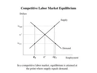
Equilibrium in a Single Competitive Labor Market • Equilibrium: • Each firm hires up to the point where • No unemployment • Anyone who wants to work at w* can • Individuals not working are looking for w_w* • Firms not finding employees are offering w_w* • Realistically, equilibrium will not last because of shocks in modern industrialized nations

Competitive Equilibrium Across Labor Markets • Labor markets may be differentiated by: • Region (north, south, etc) • Industry (2 different production industries) • Assume: • Markets in two regions (north, south) • Workers in the two regions have similar skills and can substitute for one another • Initially, ws < wn

Competitive Equilibrium Across Labor Markets, cont. • If workers have full mobility, southern workers will ___________ ____________ where they can earn a higher wage • If firms have full mobility, northern firms will _______________ where they can pay a lower wage (not shown) • In the end,

Competitive Equilibrium Across Labor Markets  Efficiency • Efficiency: • Also maximizes national income • If ws < wn, VMPs _ VMPn since profit-maximizing firms hire up to the point where • As workers migrate north, MPn_ and MPs_ until the two are equated, and • In the end, ___________________, and profits are maximized

Empirical Evidence • Do wages equate over time? • In the US, there is a strong ____________ correlation between wages and annual growth of wages • Roughly 30% of the wage gap between states disappeared over a 30-year period (states with lowest wages had highest growth rate) • Similar evidence in Japan, a less mobile country • Across countries: “Conditional convergence” • Does not apply to the wage gap between the rich and poor countries because countries with lower human capital levels do not grow as rapidly

NAFTA: Mexico and the US • Mobility of firms should: • __crease demand for Mexican workers • __crease demand for US workers with similar skills • Eventually _______ wages across the two countries • Some workers will clearly benefit and some will be harmed, but the total income of the two countries should increase as North America moves to a more __________ outcome

Policy Application: Payroll Tax • Payroll tax • Employers pay a tax on total wage bill • Employers who first paid w1 will now be willing to pay only _____ to E1 workers • _____ward shift of labor demand curve • New wage paid to workers: • Firms pay _____, because they pay tax t to the government • ______ workers hired (E2 _ E1) • Tax burden • Firms: • Employees:

Policy Application: Employee Tax • Tax on workers • E1 workers first earned w1, • Workers now demand ______ • ______ward shift of labor supply curve • New wage is ____ • Workers earn _____, because they pay tax t to government • _____ workers hired (E2 _ E1) • Tax burden • Firms: • Employees:

Tax policy application: Summary • Note that the outcome is the same regardless of who is taxed • Employee Tax: • w_, so ______ bears the cost by having to ________________ • Full amount of tax not recovered for ________ (tax is greater than the wage increase) • Payroll Tax: • w_, so _______bear the cost by ____________ • Full amount of tax is not covered for ___________ by the wage decrease (tax is greater than the wage decrease)

Tax with no burden on the firm • Assume firm is taxed • Assume perfectly inelastic supply • With tax, firm is only willing to pay ______ • Number of workers ________ _____________ • Firm passes entire incidence of the tax onto workers • Therefore, a more ________ supply curve passes more tax burden onto employees • Recall that labor supply curve for men is inelastic

Empirical Example • Note: Evidence suggests firms pass approximately 90% of tax burden onto employees • Suppose annual income = $30,000 • Employee tax = 7.65%  $2295 annually • Employer tax = 7.65%  $2295 annually • 90% of tax shifted to worker: .9·2295 = $2066 • Total employee tax = $2295 + 2066 = $4361 annually • If $4361 were invested annually at 3%, worker would accumulate $263,675 by age 65 • If worker lives to age 80, would need SS benefits of $21,000 annually • Average worker only receives $7,200

Policy Application: Government subsidy paid to employers • Subsidy lowers the cost of hiring workers • Firms are willing to pay ______ (s recouped in the form of the subsidy, so in essence, the firm is only paying original wage, w1) • New wage paid to worker: __ • Cost of employment for the firm: _______ • Benefits of subsidy • Firm: • Worker:

Empirical Example • Assume: • Elasticity of demand = -0.5 • Elasticity of supply = 0.3 • A 10% subsidy (reduction in hiring costs) would: • Increase wage by 4% • Increase employment by 2% • Gains of a government subsidy may be limited • Firms may be unaware of programs • Firms may place a stigma on hiring targeted workers and do not hire them even to benefit from employer subsidy programs

Noncompetitive Labor Markets: Monopsony • So far, competitive firms took p and w as given regardless of E* • Recall that perfectly competitive firms face a horizontal demand curve given by the market price • Analogously, an individual firm faces a horizontal labor supply curve, given w • It can hire as many workers as it long as it pays wage = w • Monopsony: • Must pay higher wages to attract more workers (p taken as given) • Note that all markets have upward-sloping supply curves, but monopsonies are firms that face upward-sloping supply curves • Ex: one-company town

Perfectly discriminating monopsonist • Monopsonist can hire different workers at different wages • w15 for worker 15, • w20 for worker 20, etc. • Supply curve = ____ • Wage paid for each worker is his ______ ____________ • Demand curve = ______ • Price is taken as given • Firm hires up to the point where _____ ____ (E*,w*), or where _____ = ______ • Same __ as a competitive market, but __ is the wage for the last worker, and all others were paid w _ w*

Non-discriminating Monopsonist • Monopsonist pays all workers the same wage, regardless of their reservation wages • Supply ≠ MC, but MC __creases as E increases • S _ MC • If the 9th worker costs $7, total labor bill = $63 • If 10th worker demands $7.50, total labor bill = $75 • MC of the 10th worker is $12, but wage was $7.50 • Analogous to D > MR for a monopolist

Non-discriminating Monopsonist, cont. • Firms hire up to the point where ___ = ____ (EM,wM) • Monopsonist determines wage from _______ curve, not MCE curve • Similar to how monopolists choose P from the demand curve, not MR • EM _ EC and wM _ wC

Monopsony and Minimum Wage • Set wmin > wM, and firm can hire E* employees • MC = wmin up to E* employees, then returns to MC curve above supply curve • Firm wants to hire where ______ = _____, which is E* employees (point A) at min wage, wmin • Outcome: wmin _ wM and E* _ EM- no unemployment • Better outcome: set wmin = __ so E = __ and w = __ • Minimum wage law outcomes may be explained by fast food restaurants acting as monopolists to teenagers

Competitive firms facing upward-sloping supply curves • Even if employees are mobile, the costs associated with moving to take advantage of a new higher paying job can be huge • Competitive firms must offer large wages to attract someone to move • As the number of employees increases, monitoring workers to discourage shirking becomes expensive • Employers may want to pay higher wages to make the cost to an employee of shirking more expensive

Professional Athletes • Free agency • If a player can go where he wants, he will present his current team with an outside offer • Current team evaluates VMP, and if VMP exceeds offer, • If not, • No free agency • New team can offer current team a trade – pay salary + bonus to total their value for the player • Current team evaluates VMP and agrees to trade if • If VMP exceeds offer,

Professional Athletes, cont. • Allocation of resources (players) • Player may not be paid according to worth, but he ends up with the team that values him the most (VMP) in either case • Different income distribution • __________ benefits from no free agency, but ________ benefits as a free agent • Empirical evidence: supports migration and income distribution predictions

Noncompetitive Labor Markets: Monopoly • Monopoly: • Recall: Monopsonist did not control p, but could choose w

Monopoly, cont. • When output increases, monopolist must ______ price on that unit and all previous units • MR _ P, where P is represented by ______ since the firm chooses P* from demand curve after Q* is chosen (MR=MC) • Competitive outcome: ______ • PC _ PM and QC _ QM

Monopoly, cont. • Since P≠MR, revenue generated by last worker hired is not equal to MPE·P = VMPE • Instead, marginal revenue product = MRPE = • MPRE _ VMPE because MR < P • π-max: w = ___, not w = VMP • EM _ EC, where EC is found be equating wage to value of marginal product

Empirical Evidence • Monopolists and oligopolists (few firms produce all of the output for an entire market) pay higher wages than competitive firms (approximately 10% more) • Monopolists can pass high production costs onto consumers, so with little incentive to keep costs down, monopolists must pay high wages for the most desirable workers

Labor Market Equilibrium