Download
1 / 33
330 likes | 437 Vues
Explore the significance of antiproton source advancements, focusing on Stochastic Cooling and high luminosity beams for Run II goals. Learn about the physics principles like Hamiltonian of charged particles, solutions to Equations of Motion, and beam size considerations. Delve into Longitudinal Effects, Debuncher Ring, Accumulator Ring, and Stochastic Cooling techniques in Pbar Storage Rings. Discover the mechanisms behind Stochastic Cooling, Betatron Cooling, and Momentum Cooling in the Pbar Source.

E N D
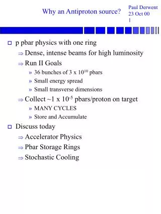
Why an Antiproton source? • p pbar physics with one ring • Dense, intense beams for high luminosity • Run II Goals • 36 bunches of 3 x 10¹⁰ pbars • Small energy spread • Small transverse dimensions • Collect ~1 x 10⁻⁵ pbars/proton on target • MANY CYCLES • Store and Accumulate • Discuss today • Accelerator Physics • Pbar Storage Rings • Stochastic Cooling
Some Necessary Accelerator Physics • All Classical (Relativistic) E&M • Hamiltonian of a charged particle in EM field • Small angle approximation around CENTRAL ORBIT • Set of Conjugate variables: • x, x’ horizontal displacement and angle • y, y’ vertical displacement and angle • E, s energy and longitudinal position • s = bct sometimes use t instead • Equation of Motion: • C is circumference of accelerator -- Periodicity!
Solutions to Equations of Motion • Restoring force k(s) is dependent on location • Dipoles • Quadrupoles • Drifts • General Solution: • b(s) is solution to a messy 2nd order Diff Eqn • Beam size depends on Amplitude of oscillation and value of b(s) • Can change Position by changing angle 90 upstreamused for extraction/injection/cooling/IP position
Beam Size • Relate the INVARIANT EMITTANCE (phase space area) to physical size • Gaussian Beams • 95% (Fermi Standard) • s2 = eb / 6p • Include relativistic contraction (beams gets smaller as they are accelerated!) • At B0: b(s) = b*(1+s2/b*2) • For 20p mm mr beams at IP • s= (20p x10-6 m r * 0.35 m / 6pg)1/2 = 3.5 x 10⁻⁵ m = 35 mm
Longitudinal Effects • Longitudinal Acceleration • Time Varying Fields to get net acceleration • Synchronous PHASE and Particle • Path Length can depend on ENERGY • Revolution Frequency can depend on ENERGY • Expressed via Phase Slip Factor h • gt transition energy • Accelerating phase needs to change by 180° as cross transition
Final Points • Frequency Spectrum • Time Domain: (t+nT0) at pickup • Frequency Domain:harmonics of revolution frequency f0 = 1/T0 • Accumulator:T0~1.6 sec (1e10 pbar = 1 mA)f0 (core) 628955 Hz 127th Harmonic ~79 MHz
Pbar Storage Rings • Two Storage Rings in Same Tunnel • Debuncher • Larger Radius • ~few x 107 stored for cycle length • 2.4 sec for MR, 1.5 sec for MI • ~few x 10-7 torr • RF Debunch beam • Cool in H, V, p • Accumulator • ~1012 stored for hours to days • ~few x 10-10 torr • Stochastic stacking • Cool in H, V, p • Both Rings are ~triangular with six fold symmetry
E t E t Debuncher Ring • Main Purpose: • “Debunch” RF Time Structure (84 buckets)RF locked to Main Injector • Rotation in Phase Space • DE, Dt conjugate variables • Initial large DE (off target), small Dt (RF) • 5 MV RF in ~1/4 turn down to ~100 kV • Small DE, large Dt • Adiabatically turn off RF (~10 msec) • Lots of time left (1.5 sec cycle) • Cool in H, V, p
Power (dB) Core Stacktail Frequency (~Energy) Injected Pulse Accumulator Ring • Not possible to continually inject beam • Violates Phase Space Conservation • Need another method to accumulate beam • Inject beam, move to different orbit (different place in phase space), stochastically stack • RF Stack Injected beam • Bunch with RF (2 buckets) • Change RF frequency (but not B field) • ENERGY CHANGE • Decelerates ~ 30 MeV • Stochastically cool beam to core • Decelerates ~60 MeV
x’ x x’ x Idea Behind Stochastic Cooling • Phase Space compression Dynamic Aperture: Area where particles can orbit Liouville’s Theorem: Local Phase Space Density for conservative system is conserved Continuous Media Discrete Particles Swap Particles and Empty Area -- lessen physical area occupied by beam
Particle Trajectory Kicker Idea Behind Stochastic Cooling • Principle of Stochastic cooling • Applied to horizontal btron oscillation • A little more difficult in practice. • Used in Debuncher and Accumulator to cool horizontal, vertical, and momentum distributions • COOLING? Temperature ~ <Kinetic Energy>minimize transverse KE minimize DE longitudinally
Stochastic Coolingin the Pbar Source • Standard Debuncher operation: • 108 pbars, uniformly distributed • ~600 kHz revolution frequency • To individually sample particles • Resolve 10-14 seconds…100 THz bandwidth • Don’t have good pickups, kickers, amplifiers in the 100 THz range • Sample Ns particles -> Stochastic process • Ns = N/2TW where T is revolution time and W bandwidth • Measure <x> deviations for Ns particles • Higher bandwidth the better the cooling
Betatron Cooling With correction ~ g<x>, where g is gain of system • New position: x - g<x> • Emittance Reduction: RMS of kth particle • Add noise (characterized by U = Noise/Signal) • Add MIXING • Randomization effects M = number of turns to completely randomize sample
Momentum Cooling • Momentum Cooling explained in context of Fokker Planck Equation • Case 1: Flux = 0 Restoring Force a(E-E0) Diffusion = D0 • Cooling of momentum distribution (as in debuncher) • ‘Small’ group with Ei-E0 >> D0 • Forced into main distribution • MOMENTUM STACKING
y ‘Stacked’ E0 Stochastic Stacking Gaussian Distribution • CORE • Injected Beam (tail) • Stacked
Upgrades for Run II • Debuncher • All stochastic cooling systems • Larger bandwidth (4-8 GHz vs. 2-4 GHz) • All new electronics and signal transmission • Lower Noise (Liquid Helium vs. Liquid Nitrogen) • Different Technology • Slot coupled waveguides vs. Octave bandwidth pickups • Remove H & V trim magnets to make room for cooling tanks • Move quadrupoles for use in steering • Adjust quad positions in D-to-A line to make room for cooling tanks
Beam Direction Slot Coupled Waveguides Output Port Output Termination Output Port Output Termination • Slot Coupled Waveguide an electromagnetic whistle • Narrow Band (~0.5 GHz), High Sensitivity • Cover 4 bands (2 GHz bandwidth)
Debuncher Upgrade • Slot Coupled Waveguide • Narrow Band (~0.5 GHz), High Sensitivity • Cover 4 bands (2 GHz bandwidth)
Debuncher Upgrade • Slow Wave Structure: size, spacing, and number of slots determines sensitivity and bandwidth
Debuncher Upgrades • 4 Kicker bands • 8 Pickup bands
Debuncher Momentum Cooling Blue Trace: Debuncher Momentum Cooling Off Orange Trace: Debuncher Momentum Cooling On Beam on Accumulator Injection Orbit
Debuncher Signal to Noise • For Horizontal Band 1 • Signal to Noise for 1e7 particles (expect 8e7 during Run II) • Room Temperature (red), He Temperature (blue/purple)
Gain Density Stacktail Core Stacktail Core Energy Energy Stochastic Stacking • Simon van Der Meer solution: • Constant Flux: • Solution: • Exponential Density Distribution generated by Exponential Gain Distribution Using log scales on vertical axis
Implementation in Accumulator • Stacktail and Core systems • How do we build an exponential gain distribution? • Beam Pickups: • Charged Particles: E & B fields generate image currents in beam pipe • Pickup disrupts image currents, inducing a voltage signal • Octave Bandwidth (1-2, 2-4,4-8 GHz) • Output is combined using binary combiner boards to make a phased antenna array
Planar Loops 3D Loops Beam Pickups Pickup disrupts image currents, inducing a voltage signal
I A Beam Pickups • At A:Current induced by voltage across junction splits in two, 1/2 goes out, 1/2 travels with image current
Beam Pickups • At B:Current splits in two paths, now with OPPOSITE sign • Into load resistor ~ 0 current • Two current pulses out signal line I B DT = L/bc
Beam Pickups • Current intercepted by pickup: • Use method of images • Placement of pickups to give proper gain distribution -w/2 +w/2 y d x Dx Current Distribution
Accumulator Pickups • Placement, number of pickups, amplification are used to build gain shape Core = A - B Stacktail Energy Gain Core Stacktail Energy
Accumulator Upgrades for Run II • Accumulator • Stacktail Stochastic Cooling Systems • Larger Bandwidth (2-4 GHz vs. 1-2 GHz) • New technologies for signal combination • Recycled (from Debuncher) and new Electronics to cover larger bandwidth • Lattice changes • Halve phase slip factor (h) • Driven by Stacktail upgrade • Keep dispersion, phase advance (pickup to kicker) injection and extraction regions, tunes, aperture, chromaticity ~ the same • Requires construction 4 new quadrupoles (strength vs. current characteristics) • Reworking of power supplies
Why change h? f/f = p/p = h/DDx/x Momentum Spread~100 MeV Frequency Spread ~ 160 Hz fcentral ~ 628900 Hz f /f ~ 2.5e-4 Stacktail assumes position(energy) frequency relation in design 1 GHz ~ 1590 Harmonic f ~ 254000 Hz 2 GHz ~ 3180 Harmonic f ~ 508000 Hz 3 GHz ~ 4770 Harmonic f ~ 763000 Hz Frequency Spread > harmonic frequency! Frequency Energy Map no longer 1 1
Accumulator Stacktail Performance with Protons • Inject 8 GeV protons • ‘Stacking’ rate ~ 13 mA/hour!
AntiProton Source • Shorter Cycle Time in Main Injector • Target Station Upgrades • Debuncher Cooling Upgrades • Accumulator Cooling Upgrades • GOAL: >20 mA/hour