Linear Prediction
Linear Prediction. Linear Prediction (Introduction) :. The object of linear prediction is to estimate the output sequence from a linear combination of input samples, past output samples or both : The factors a(i) and b(j) are called predictor coefficients.

Linear Prediction
E N D
Presentation Transcript
Linear Prediction (Introduction): • The object of linear prediction is to estimate the output sequence from a linear combination of input samples, past output samples or both : • The factors a(i) and b(j) are called predictor coefficients.
Linear Prediction (Introduction): • Many systems of interest to us are describable by a linear, constant-coefficient difference equation : • If Y(z)/X(z)=H(z), where H(z) is a ratio of polynomials N(z)/D(z), then • Thus the predictor coefficients give us immediate access to the poles and zeros of H(z).
Linear Prediction (Types of System Model): • There are two important variants : • All-pole model (in statistics, autoregressive (AR) model ) : • The numerator N(z) is a constant. • All-zero model (in statistics, moving-average(MA) model ) : • The denominator D(z) is equal to unity. • The mixed pole-zero model is called the autoregressive moving-average(ARMA) model.
Linear Prediction (Derivation of LP equations): • Given a zero-mean signal y(n), in the AR model : • The error is : • To derive the predictor we use the orthogonality principle, the principle states that the desired coefficients are those which make the error orthogonal to the samples y(n-1), y(n-2),…, y(n-p).
Linear Prediction (Derivation of LP equations): • Thus we require that • Or, • Interchanging the operation of averaging and summing, and representing < > by summing over n, we have • The required predictors are found by solving these equations.
Linear Prediction (Derivation of LP equations): • The orthogonality principle also states that resulting minimum error is given by • Or, • We can minimize the error over all time : • where
σ 1-A(z) Linear Prediction (Applications): • Autocorrelation matching : • We have a signal y(n) with known autocorrelation . We model this with the AR system shown below :
Linear Prediction (Order of Linear Prediction): • The choice of predictor order depends on the analysis bandwidth. The rule of thumb is : • For a normal vocal tract, there is an average of about one formant per kilo Hertz of BW. • One formant requires two complex conjugate poles. • Hence for every formant we require two predictor coefficients, or two coefficients per kilo Hertz of bandwidth.
Linear Prediction (AR Modeling of Speech Signal): • True Model: Pitch Gain s(n) Speech Signal DT Impulse generator G(z) Glottal Filter Voiced U(n) Voiced Volume velocity H(z) Vocal tract Filter R(z) LP Filter V U Uncorrelated Noise generator Unvoiced Gain
Linear Prediction (AR Modeling of Speech Signal): • Using LP analysis : Pitch Gain estimate DT Impulse generator Voiced s(n) Speech Signal All-Pole Filter (AR) V U White Noise generator Unvoiced H(z)