Galerkin’s Method for Differential Equation
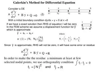
Galerkin’s Method for Differential Equation. (I). In order to make the the residue a minimum at least at few selected nodal points, we use orthogonality condition. (II). Integrating the first term of equation II. Equation II becomes.

Galerkin’s Method for Differential Equation
E N D
Presentation Transcript
Galerkin’s Method for Differential Equation (I) In order to make the the residue a minimum at least at few selected nodal points, we use orthogonality condition
(II) Integrating the first term of equation II Equation II becomes
The first term is based on initial boundary conditions. For the given problem dy/dx is known only at x = o, and at subsequent points at x = l, 2L …. is not known and hence subsequent terms are ignored.
Using the conditions dy/dx = y1 = 0 and solving the system of equations, y2,y3, andy4 can be solved
Heat & Mass Transfer • Basic DE for one dimesion -Change in stored energy -Energy generated(source or sink) inside the control volume -Energy output from control volume S3 (area around the perimeter) S2 S1
- heat conducted(heat influx) into the control volume at surface edge x (kW/m2 or Btu/h-ft2) - heat conducted out of control volume at surface edge x+dx -the internal heat source(heat generated/unit volume) or a sink (heat drawn out of volume) (kW/m3 or Btu/h-ft3) -Area of control volume surface From Fourier’s law of heat conduction -thermal conductivity in x direction -temperature; - Temperature gradient
Using Taylor expansion: The change in stored energy: -specific heat in kWh/kg
Simplify the equation: For steady state condition: For 2 dimension case:
Heat transfer with conduction For a conducting solid in contact with fluid, there will be a heat transfer between solid and fluid. Heat flow by convection: -Heat transfer or convection coeffient -Temperature of solid surface -Temperature of liquid
One dimensional Problem 1 2 The temperature gradient matrix The heat flux/temperature gradient relationship is given by
Casting the governing DE into integral form using Galcerkin approach. The last integrand can be written as
In case the surface S2 convects heat in addition to heat flux, additional boundary Condition is required for the last element For the last element
Structural Analysis Thermal Analysis Structural vs Heat Transfer • Select element type • Select element type • Assume displacement function • Assume temperature function • Stress/strain relationships • Temperature relationships • Derive element stiffness • Derive element conduction • Assemble element equations • Assemble element equations • Solve nodal displacements • Solve nodal temperatures • Solve element forces • Solve element gradient/flux
Finite Element 2-D Conduction Assume (Choose) a Temperature Function Assume a linear temperature function for each element as: where u and v describe temperature gradients at (xi,yi). 3 Nodes 1 Element 2 DOF: x, y
Finite Element 2-D Conduction Assume (Choose) a Temperature Function
Finite Element 2-D Conduction Define Temperature Gradient Relationships Analogous to strain matrix: {g}=[B]{t} [B] is derivative of [N]
Finite Element 2-D Conduction Derive Element Conduction Matrix and Equations i h j m
Stiffness matrix is general term for a matrix of known coefficients being multiplied by unknown degrees of freedom, i.e., displacement OR temperature, etc. Thus, the element conduction matrix is often referred to as the stiffness matrix.