Download
1 / 31
510 likes | 1.01k Vues
Thermometry using Laser Induced Thermal Grating Spectroscopy (LITGS). Joveria Baig. Outline. Motivation Optical techniques Laser Induced Grating Spectroscopy Thermometry using LITGS Spatial Averaging in LITGS Sensitivity of LITGS in complex temperature fields Thermometry in burner flame

E N D
Thermometry using Laser Induced Thermal Grating Spectroscopy (LITGS) JoveriaBaig
Outline • Motivation • Optical techniques • Laser Induced Grating Spectroscopy • Thermometry using LITGS • Spatial Averaging in LITGS • Sensitivity of LITGS in complex temperature fields • Thermometry in burner flame • Outlook
Motivation The world still heavily relies on combustion of fossil fuels as a primary source of energy. • Understanding the process of combustion will help: • Reduce impact of harmful pollutants • Increase efficiency of combustion to reduce amount of fuel used Reaction rates are dependent on temperature by the Arrhenius equation: • Thermometry: • Accurate and precise • Spatially resolved where k is the reaction rate, A is a pre-factor and T is the absolute temperature
Four Wave Mixing • Generation of fourth signal field as function of three input fields • Power series expansion of polarization relates the three source fields through third order electric susceptibility tensor: • Conservation of momentum and energy dictates the phase matching criteria
Laser Induced Thermal Grating Spectroscopy Signal Formation: • Two coherent beams interfere to form intensity fringes at the intersection. • Molecular excitation, followed by collisional quenching causes a grating to form in the gas. • Bragg scattered probe beam forms the LITGS signal. Pump Thermal Grating LITGS signal Pump Probe
LITGS • Acoustic waves formed by fast release of energy from the excited molecules • Stationary wave due to change in temperature • Change in bulk gas density and hence refractive index
Thermometry using LITGS • Bragg scattered probe beam can be used to monitor the grating evolution Λ θ = angle of incidence of pump beam = ratio of mass to specific heats
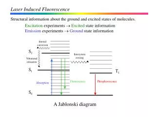
ν‘ ħω2 ħω3 ħω1 ħω4 ħω1 ħω2 ħω3 ħω4 ν Alternative optical techniques Degenerate Four Wave Mixing (DFWM) Coherent Anti-stokes Raman Spectroscopy (CARS) • Laser Induced Fluorescence (LIF) • Temperature measurement from intensity of fluorescent signal Population Grating Population Grating absorption fluorescence Laser Resonantly enhanced by real transition Absorption Spectroscopy Doppler broadened line width can give information about temperature Probe grating at same wavelength Fluorescence Probe grating at any wavelength Stationary population grating – fast decay Moving population grating
Spatial Averaging Presence of multiple temperatures in the probe volume (in non-uniform temperature fields) can significantly change the shape of LITGS signal
LITGS Experimental Setup Pump beam: • Quadrupled Nd:YAG laser (266nm) • Energy of 15 mJ Probe beam: • 300mW Continuous wave diode pumped Solid State laser
Dual Flow Experiment • To test the effect of two temperatures in the probe volume • Hot flow connected to heating element, cold flow at room temperature • Translation stages to adjust the position of the flow system relative to the optical table
Validation • Model developed for calculating LITGS signal for a uniform temperature field • Single temperature LITGS model fits well with the experimental data Dual temperature model developed to simulate LITGS signal in a probe volume containing two different temperatures
Different Temperature Distributions Hot 430K Cold 270K Hot Cold Hot Two different annular temperature distributions modelled • ‘Hot-cold-hot’ flow • ‘Cold-hot-cold’ flow
Different Temperature Distributions Hot 430K Cold 270K Two different annular temperature distributions modelled • ‘Hot-cold-hot’ flow • ‘Cold-hot-cold’ flow Cold Hot Cold
Objective Burnt gas (hot region) Un-burnt ethylene (flame front) • Evaluate what happens in a single 2D slice at different heights along in the flame • Reconstruction of temperature distribution in 3D
Model • LIGS signal at different positions show presence of multiple temperature • Frequency beating like behavior seen Figure showing temperature distribution Inner circle (cold) 270K Outer ring (hot) 430K
Power Spectrum Power spectrum shows two peak frequencies corresponding to presence of two temperatures in the distribution
Experimental Setup • Thermometry in standardized laboratory flame as a precursor to more complicated combustion processes • Co-flow laminar ethylene-air diffusion flow
Experimental data from flame • Probe region has to be greater than the flame diameter • Coarse grid of 2D slice through the flame • Measurements require ethylene hence constrained by flame front 7 cm x x x x x x x x x • Locations from where experimental data was obtained for fitting is shown by red crosses 12 mm
Results At x=0, z=0 in flame • Fast decay of the signal: • Presence of high temperature • Weighted LITGS of multiple temperatures in probe volume
Conclusion • Developed understanding of spatial averaging in LITGS • Applied to axi-symmetric flame environment • Successfully recovered temperature distribution with significantly enhanced spatial resolution by combining this new understanding of spatial averaging with object symmetry in a novel fitting approach using data from multiple chords
Future Work • Acquire experimental data at closer intervals to achieve better fitting with the current model • Model to be made more precise by optimizing parameters such as Reynolds number, quench times, branching ratio etc for each temperature • Combine with other techniques such as Chemilumiscence to get more information about flame • Incorporate details of probe volume shape