Download
1 / 35
350 likes | 486 Vues
Latent heat fluxes during stably stratified conditions. Stephan de Roode with contributions from Fred Bosveld and Reinder Ronda. Turbulent transport: Turbulent kinetic energy E > 0 For very stable conditions shear generation of TKE is not sufficient(?).

E N D
Latent heat fluxes during stably stratified conditions Stephan de Roode with contributions from Fred Bosveld and Reinder Ronda
Turbulent transport: Turbulent kinetic energy E > 0For very stable conditions shear generation of TKE is not sufficient(?) buoyancy shear production turbulent transport dissipation TKE production requires Write and if KH = KM then TKE production for the following criterion Bulk critical Richardson number
Stable boundary layersCabauw data 2000-2006 Data selection: weak winds: Utot (z=10 m) < 3 m/s clear skies: LWnet,sfc > 40 W/m2 nighttime: SWnet,sfc = 0 W/m2 7.1% of all data points satisfy these criteria
Stable boundary layersCabauw data 2000-2006 Further data selection: Latent, sensible and ground heat flow at 5 cm are available weak winds: Utot (z=10 m) < 3 m/s clear skies: LWnet,sfc > 40 W/m2 nighttime: SWnet,sfc = 0 W/m2 3.5% of all data points
Surface energy balance during the night night-time Low wind speeds during stable nights: turbulent fluxes H and LE become very small. -G = SW + LW + H + LE G = energy flow into the ground SW = net shortwave radiation LW = net longwave radiation H = sensible heat flux LE = latent heat flux (evaporation)
Cabauw Monthly Mean Surface Energy Balance results for stable boundary layers [W/m2]
Is it possible to close the surface energy balance from observations?
Dew formation in Wageningen Results based on modeling and observations from Jacobs et al. (2006)
Energy equivalence of dew formation Evaporation of 1 kg (= 1mm) of water: 2.5·106 J In Wageningen monthly mean dew formation: 3.5 mm/month = 0.12 mm/day Rough estimation: Assume that dew formation takes place during 12 hours (half a day) then the typical heat production due to dew formation amounts 2.5·106 x 0.12 / 12 / 3600 = 7 W/m2
A few examples from Cabauw • Select clear nights with low wind speeds • Select negative humidity tendencies • In the examples that will be shown the observed latent heat flux ~ 0 W/m2
Moisture tendencies: weak wind velocities qsat,sfc z=2m z=10m z=80m z=200m
Moisture tendencies: weak wind velocities qsat,sfc z=2m z=10m z=80m z=200m
Moisture tendencies: weak wind velocities qsat,sfc z=10m z=2m z=80m z=200m
Moisture tendencies: very weak wind velocities qsat,sfc z=2m z=10m z=80m z=200m
Moisture tendencies: very weak wind velocities qsat,sfc z=2m z=10m z=80m z=200m
Add selection criterion: humidity tendency < 0.02 g/kg/hour at z=20mMonthly mean humidity tendencies z=200m z=80m z=10m z=2m
Conclusions from observations • Specific humidity in the lower part of the atmosphere follows surface saturation specific humidity rather well • It is difficult to assess the magnitude of the large-scale horizontal advection of moisture • Diagnose the latent heat flux from the humidity budget equation
Latent heat fluxes diagnosed from the humidity budget equationMonthly mean values II I I. Neglect large-scale advection term II. Large-scale (ls) tendency correction. Assume that the tendency at 200 m is representative for the ls-tendency at every height.
Turbulent potential energy TPETotal turbulent energy TTE (Zilitinkevich, 2007) shear production turbulent transport total dissipation
Prognostic equations Stable <0 always >0 ! transport dissipation radiation Unstable > 0
Large eddy simulation • Initial (very) stable lapse rate: • No fluxes at the surface, no moisture present • No horizontal winds: U=V=0.001 m/s • nr of grid points Nx=Ny=64 , Nz=80 • Dx=Dy=Dz=5m • sinusoidal q initial perturbation at layers between 50 and 150 m • amplitude of perturbation qAMPL =0.5 K • What will happen?
Turbulent kinetic energy (TKE) - Turbulent potential energy (TPE) TPE (buoyancy variance term) TKE ● TKE generation by TPE, their sum is not conserved (dissipation) ● Rapid oscillations (but not Brunt-Vaissala frequency) ● vertical integral buoyancy flux > 0 for d/dt TKE > 0 and vice versa
Lorenz, Available potential energy and the maintenance of the general circulation, Tellus., 1955 Lorenz showed that available potential energy (APE) is given approximately by the volume integral over the entire atmosphere of the variance of potential temperature on isobaric surfaces: As the potential temperature is conserved for adiabatic processes, and as kinetic energy is produced, the enthalpy (cpT) of the atmosphere should decrease (see also Holton 1992)
Temperature evolution t=0 t=1200 s
Enthalpy change PKE TKE enthalpy ● Enthalpy in phase with PKE and TKE
Conclusions ● Surface energy balance does not close for Cabauw for strong stable conditions Observations suggests the observed latent heat flux is underestimated ● Concept of 'total turbulent energy' is just a smart combination of the variance equations for E and the virtual potential temperature. Note that Nieuwstadt also uses these equations and gets identical solutions as from a simple TKE equation (Baas et al., 2007) ● However, note that buoyancy fluctuations plane will trigger vertical motions ● The radiation term might be very important in generating temperature variance
Can we measure small latent heat fluxes? Write the flux according to an updraft downdraft decomposition: with s = updraft fraction wu (wd) = updraft (downdraft) vertical velocity qu (qd) = updraft (downdraft) specific humidity
Can we measure small latent heat fluxes? Measure 7 W/m2: Examples wu (m/s) qt' (g/kg) 1 0.0028 0.1 0.028 0.001 0.28 Li-Cor Li7500 RMS noise ± 0.0033 g/kg
Soil heat flux Soil heat flux: soil heat flux plates. The six plates are burried at the three vertices of an equilateral triangle with sides of 2 m at depths of 0.05 and 0.10 m. The measurements are averaged over the three plates at each depth. To obtain the surface soil heat flux a Fourier decompostion method is used. The instruments are manufactured by TNO-Delft. Type: WS31S, measuring principle: thermo-pile, diameter 0.11 m, thickness 5 mm, sensitive surface: central square of 25*25 mm2. Thermal conductivity of the sensor 0.2-0.3 W/m/K.
Temperature tendencies during stable, clear nights:Monthly mean values [K/hour]
Humidity tendencies during stable, clear nights:Monthly mean values [g/kg/hour]
Humidity budget equationI. Neglect large-scale advection termII. Assume 200 m tendency is due to horizontal advection