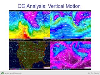
QG Analysis: Vertical Motion
QG Analysis: Vertical Motion. QG Analysis. QG Theory Basic Idea Approximations and Validity QG Equations / Reference QG Analysis Basic Idea Estimating Vertical Motion QG Omega Equation: Basic Form QG Omega Equation: Relation to Jet Streaks QG Omega Equation: Q-vector Form

QG Analysis: Vertical Motion
E N D
Presentation Transcript
QG Analysis: Vertical Motion M. D. Eastin
QG Analysis • QG Theory • Basic Idea • Approximations and Validity • QG Equations / Reference • QG Analysis • Basic Idea • Estimating Vertical Motion • QG Omega Equation: Basic Form • QG Omega Equation: Relation to Jet Streaks • QG Omega Equation: Q-vector Form • Estimating System Evolution • QG Height Tendency Equation • Diabatic and Orographic Processes • Evolution of Low-level Cyclones • Evolution of Upper-level Troughs M. D. Eastin
QG Analysis: Basic Idea • Forecast Needs: • The public desires information regarding temperature, humidity, precipitation, • and wind speed and direction up to 7 days in advance across the entire country • Such information is largely a function of the evolving synoptic weather patterns • (i.e., surface pressure systems, fronts, and jet streams) • Forecast Method: • Kinematic Approach: Analyze current observations of wind, temperature, and moisture fields • Assume clouds and precipitation occur when there is upward motion • and an adequate supply of moisture • QG theory • QG Analysis: • Vertical Motion: Diagnose synoptic-scale vertical motion from the observed • distributions of differential geostrophic vorticity advection • and temperature advection • System Evolution: Predict changes in the local geopotential height patterns from • the observed distributions of geostrophic vorticity advection • and differential temperature advection M. D. Eastin
QG Analysis: Basic Idea • Estimating vertical motion in the atmosphere: • Our Challenge: • We do not observe vertical motion • Vertical motions influence clouds and precipitation • Actual vertical motions are often several orders of magnitude smaller • than their collocated horizontal air motions [ w ~ 0.01 → 10 m/s ] • [ u,v ~ 10 → 100 m/s ] • Synoptic-scale vertical motions must be estimated from widely-spaced • observations (i.e., the rawinsonde network) every 12-hours • Methods: • Kinematic Method Integrate the Continuity Equation • Very sensitive to small errors in winds measurements • Adiabatic Method From the thermodynamic equation • Very sensitive to temperature tendencies (difficult to observe) • Difficult to incorporate impacts of diabatic heating • QG Omega Equation Least sensitive to small observational errors Widely believed to be the best method M. D. Eastin
QG Analysis: A Closed System of Equations • Two Prognostic Equations – We Need Two Unknowns: • In order to analyze vertical motion, we need to combine our two primary prognostic • equations – for ζgand T – into a single equation for ω • These 2 equations have 3 prognostic variables (ζg, T, and ω) → we want to keep ω • We need to convert both ζg and T into a common prognostic variable • Common Variable: Geopotential-Height Tendency (χ): • We define a local change (or tendency) in geopotential-height: • where Vorticity Equation Adiabatic Thermodynamic Equation M. D. Eastin
QG Analysis: A Closed System of Equations • ExpressingVorticityin terms of Geopotential Height: • Begin with the definition of geostrophic relative vorticity: • where • Substitute using the geostrophic wind relations, and one can easily show: • where • We can now define local changes in geostrophic vorticity in terms of geopotential • height and local height tendency (on pressure surfaces) M. D. Eastin
QG Analysis: A Closed System of Equations • ExpressingTemperaturein terms of Geopotential Height: • Begin with the hydrostatic relation in isobaric coordinates: • Using some algebra, one can easily show: • We can now define local changes in temperature in terms of geopotential height • and local height tendency (on pressure surfaces) M. D. Eastin
QG Analysis: A Closed System of Equations • Two Prognostic Equations – We Need Two Unknowns: • We can now used these relationships to construct a closed system with two prognostic • equations and two prognostic variables: Note: These two equations will used to obtain the QG omega equation and, eventually, the QG height-tendency equation M. D. Eastin
QG Analysis: Vertical Motion • The QG Omega Equation: • We can also derive a singlediagnostic equation for ω by combining our modified • vorticity and thermodynamic equations (the height-tendency versions): • To do this, we need to eliminate the height tendency (χ) from both equations • Step 1: Apply the operator to the vorticity equation • Step 2: Apply the operator to the thermodynamic equation • Step 3: Subtract the result of Step 1 from the result of Step 2 • After a lot of math, we get the resulting diagnostic equation…… M. D. Eastin
QG Analysis: Vertical Motion • The QG Omega Equation: • This is (2.29) in the Lackmann text • This form of the equation is not very intuitive since we transformed geostrophic • vorticity and temperature into terms of geopotential height. • To make this equation more intuitive, let’s transform them back… M. D. Eastin
QG Analysis: Vertical Motion • The BASICQG Omega Equation: • Term ATerm BTerm C • To obtain an actual value for ω (the ideal goal), we would need to compute the • forcing terms (Terms B and C) from the three-dimensional wind and temperature fields, • and then invert the operator in Term A using a numerical procedure, called “successive • over-relaxation”, with appropriate boundary conditions • This is NOT a simple task (forecasters never do this)….. • Rather, we can infer the sign and relative magnitude of ω through simple inspection • of the three-dimensional absolute geostrophic vorticity and temperature fields • (forecasters do this all the time…) • Thus, let’s examine the physical interpretation of each term…. M. D. Eastin
QG Analysis: Vertical Motion • The BASIC QG Omega Equation: • Term ATerm BTerm C • Term A: Local Vertical Motion • This term is our goal – a qualitative estimate of the deep–layer • synoptic-scale vertical motion at a particular location • For synoptic-scale atmospheric waves, this term is proportional to –ω • Given that ω is negative for upward motion, conveniently, –ω has the same sign • as the height coordinate upward motion +w • Thus, if we incorporate the negative sign into our physical interpretation, • we can just think of this term as “traditional” vertical motion M. D. Eastin
QG Analysis: Vertical Motion • The BASIC QG Omega Equation: • Term ATerm BTerm C • Term B: Vertical Derivative of Absolute Geostrophic Vorticity Advection • (Differential Vorticity Advection) • Single Pressure Level: • Positive vorticity advection (PVA) PVA → • causes local vorticity increases • From our relationship between ζg and χ, we know that PVA is equivalent to: • therefore: PVA → or, since: PVA → • Thus, we know that PVAat a single level leads toheight falls • Using similar logic, NVA at a single level leads to height rises M. D. Eastin
QG Analysis: Vertical Motion • The BASIC QG Omega Equation: • Term ATerm BTerm C • Term B: Vertical Derivative of Absolute Geostrophic Vorticity Advection • (Differential Vorticity Advection) • Multiple Pressure Levels • Consider a three-layer atmosphere where PVA is strongest in the upper layer: • WAIT! Hydrostatic balance (via the hypsometric equation) requires ALL changes • in thickness (ΔZ) to be accompanied by temperature changes. • BUT these thickness changes were NOT a result of temperature changes… Z-top Upper Surfaces Fell More PVA Z-400mb Pressure Surfaces Fell PVA ΔZ ΔZ decreases Z-700mb Thickness Changes PVA ΔZ ΔZ decreases Z-bottom M. D. Eastin
QG Analysis: Vertical Motion • The BASIC QG Omega Equation: • Term ATerm BTerm C • Term B: Vertical Derivative of Absolute Geostrophic Vorticity Advection • (Differential Vorticity Advection) • In order to maintain hydrostatic balance, any thickness decreases must be • accompanied by a temperature decrease or cooling • Recall our adiabatic assumption • Therefore, in the absence of temperature advection and diabatic processes: • An increase in PVA with height will induce rising motion Adiabatic Cooling Adiabatic Warming Rising Motions Sinking Motions M. D. Eastin
QG Analysis: Vertical Motion • The BASIC QG Omega Equation: • Term ATerm BTerm C • Term B: Vertical Derivative of Absolute Geostrophic Vorticity Advection • (Differential Vorticity Advection) • Possible rising motion scenarios: Strong PVA in upper levels • Weak PVA in lower levels • PVA in upper levels • No vorticity advection in lower levels • PVAin upper levels • NVA in lower levels • Weak NVA in upper levels • Strong NVA in lower levels M. D. Eastin
QG Analysis: Vertical Motion • The BASIC QG Omega Equation: • Term ATerm BTerm C • Term B: Vertical Derivative of Absolute Geostrophic Vorticity Advection • (Differential Vorticity Advection) • Multiple Pressure Levels • Consider a three-layer atmosphere where NVA is strongest in the upper layer: • WAIT! Hydrostatic balance (via the hypsometric equation) requires ALL changes • in thickness (ΔZ) to be accompanied by temperature changes. • BUT these thickness changes were NOT a result of temperature changes… Upper Surfaces Rose More Z-top NVA Z-400mb Pressure Surfaces Rose ΔZ increases NVA ΔZ Z-700mb ΔZ increases Thickness Changes NVA ΔZ Z-bottom M. D. Eastin
QG Analysis: Vertical Motion • The BASIC QG Omega Equation: • Term ATerm BTerm C • Term B: Vertical Derivative of Absolute Geostrophic Vorticity Advection • (Differential Vorticity Advection) • In order to maintain hydrostatic balance, any thickness increases must be • accompanied by a temperature increase or warming • Recall our adiabatic assumption • Therefore, in the absence of temperature advection and diabatic processes: • An increase in NVA with heightwill induce sinking motion Adiabatic Cooling Adiabatic Warming Rising Motions Sinking Motions M. D. Eastin
QG Analysis: Vertical Motion • The BASIC QG Omega Equation: • Term ATerm BTerm C • Term B: Vertical Derivative of Absolute Geostrophic Vorticity Advection • (Differential Vorticity Advection) • Possible rising motionscenarios: Strong NVA in upper levels • Weak NVA in lower levels • NVA in upper levels • No vorticity advection in lower levels • NVAin upper levels • PVA in lower levels • Weak PVAin upper levels • Strong PVA in lower levels M. D. Eastin
QG Analysis: Vertical Motion The BASIC QG Omega Equation: Term B: Vertical Derivative of Absolute Geostrophic Vorticity Advection (Differential Vorticity Advection) Full-Physics Model Analysis Strong PVA Weaker PVA below (not shown) Expect Rising Motion Strong NVA Weaker NVA below (not shown) Expect Sinking Motion M. D. Eastin
QG Analysis: Vertical Motion The BASIC QG Omega Equation: Term B: Vertical Derivative of Absolute Geostrophic Vorticity Advection (Differential Vorticity Advection) Generally consistent with expectations! Expected Rising Motion Expected Sinking Motion M. D. Eastin
QG Analysis: Vertical Motion • The BASIC QG Omega Equation: • Term B: Vertical Derivative of Absolute Geostrophic Vorticity Advection • (Differential Vorticity Advection) • Generally Consistent…BUT Noisy → Why? • Only evaluated one level (500mb) → should evaluate multiple levels • Used full wind and vorticity fields → should use geostrophic wind and vorticity • Mesoscale-convective processes → QG focuses on only synoptic-scale (small Ro) • Condensation / Evaporation → neglected diabatic processes • Complex terrain → neglected orographic effects • Did not consider temperature (thermal) advection (Term C)!!! • Yet, despite all these caveats, the analyzed vertical motion pattern is • qualitatively consistent with expectations from the QG omega equation!!! M. D. Eastin
QG Analysis: Vertical Motion • The BASIC QG Omega Equation: • Term ATerm BTerm C • Term C: Geostrophic Temperature Advection (Thermal Advection) • Warm air advection (WAA) leads to local temperature / thickness increases • Consider the three-layer model, with WAA strongest in the middle layer • WAIT! Local geopotential height rises (falls) produce changes in the local height • gradients → changing the local geostrophic wind and vorticity • BUT these thickness changes were NOT a result of geostrophic vorticity changes… Z-top Surface Rose Z-400mb WAA ΔZ ΔZ increases Surface Fell Z-700mb Z-bottom M. D. Eastin
QG Analysis: Vertical Motion • The BASIC QG Omega Equation: • Term ATerm BTerm C • Term C: Geostrophic Temperature Advection (Thermal Advection) • In order to maintain geostrophic flow, any thickness changes must be accompanied • by ageostrophic divergence (convergence) in regions of height rises (falls), which • via mass continuity requires a vertical motion through the layer • Therefore, in the absence of geostrophic vorticity advection and diabatic processes: • WAA will induce rising motion Z-top Z-top Surface Rose QG Mass Continuity Z-400mb Z-400mb ΔZ increase Surface Fell Z-700mb Z-700mb Z-bottom Z-bottom M. D. Eastin
QG Analysis: Vertical Motion • The BASIC QG Omega Equation: • Term ATerm BTerm C • Term C: Geostrophic Temperature Advection (Thermal Advection) • Cold air advection (CAA) leads to local temperature / thickness decreases • Consider the three-layer model, with CAA strongest in the middle layer • WAIT! Local geopotential height rises (falls) produce changes in the local height • gradients → changing the local geostrophic wind and vorticity • BUT these thickness changes were NOT a result of geostrophic vorticity changes… Z-top Surface Fell Z-400mb ΔZ decreases CAA ΔZ Z-700mb Surface Rose Z-bottom M. D. Eastin
QG Analysis: Vertical Motion • The BASIC QG Omega Equation: • Term ATerm BTerm C • Term C: Geostrophic Temperature Advection (Thermal Advection) • In order to maintain geostrophic flow, any thickness changes must be accompanied • by ageostrophic divergence (convergence) in regions of height rises (falls), which • via mass continuity requires a vertical motion through the layer • Therefore, in the absence of geostrophic vorticity advection and diabatic processes: • CAA will induce sinking motion QG Mass Continuity Z-top Z-top Surface Fell Z-400mb Z-400mb ΔZ decrease Z-700mb Z-700mb Surface Rose Z-bottom Z-bottom M. D. Eastin
QG Analysis: Vertical Motion The BASIC QG Omega Equation: Term C: Geostrophic Temperature Advection (Thermal Advection) Full-Physics Model Analysis Strong WAA Expect Rising Motion Strong CAA Expect Sinking Motion M. D. Eastin
QG Analysis: Vertical Motion The BASIC QG Omega Equation: Term C: Geostrophic Temperature Advection (Thermal Advection) Somewhat consistent with expectations… Strong WAA Expected Rising Motion Strong CAA Expected Sinking Motion M. D. Eastin
QG Analysis: Vertical Motion • The BASIC QG Omega Equation: • Term C: Geostrophic Temperature Advection (Thermal Advection) • Somewhat Consistent…BUT very noisy → Why? • Used full wind field → should use geostrophic wind • Only evaluated one level (850mb) → should evaluate multiple levels • Mesoscale-convective processes → QG focuses on only synoptic-scale (small Ro) • Condensation / Evaporation→ neglected diabatic processes • Complex terrain → neglected orographic effects • Did not consider differential vorticity advection (Term B)!!! • Yet, despite all these caveats, the analyzed vertical motion pattern is still • somewhat consistent with expectations from the QG omega equation!!! M. D. Eastin
QG Analysis: Vertical Motion • The BASIC QG Omega Equation: • Term ATerm BTerm C • Application Tips: • Remember the underlying assumptions!!! • You must consider the effects of bothTerm B and Term C at multiple levels!!! • If differential vorticity advection is large (small), then you should expect • a correspondingly large (small) vertical motion through that layer • The stronger the temperature advection, the stronger the vertical motion • If WAA (CAA) is observed at several consecutive pressure levels, expect a deep layer of rising (sinking) motion • Opposing expectations from the two terms at a given location will weaken the total vertical motion (and complicate the interpretation)!!! [more on this later] M. D. Eastin
QG Analysis: Vertical Motion • The BASIC QG Omega Equation: • Term ATerm BTerm C • Application Tips: • The QG omega equation is a diagnosticequation: • The equation does notpredict future vertical motion patterns • The forcing functions (Terms B and C) produce instantaneous responses • Use of the QG omega equation in a diagnostic setting: • Diagnose the synoptic–scale vertical motion pattern, and assume rising motion • corresponds to clouds and precipitation when ample moisture is available • Compare to the observed patterns → can infer mesoscale contributions • Helps distinguish between areas of persistent light precipitation (synoptic-scale) • and more sporadic intense precipitation (mesoscale) M. D. Eastin
QG Analysis: Application to Jet Streaks • Review of Jet Streaks: • Air parcels accelerate just upstream into • the “entrance” region and then decelerate • downstream coming out of the “exit” region • (for an observer facing downstream) • Often sub-divided into quadrants: • Right Entrance (or R-En) • Left Entrance (or L-En) • Right Exit (or R-Ex) • Left Exit (or L-Ex) • Each quadrant has an “expected” vertical motion….WHY? Left Exit Left Entrance Descent Ascent Jet Streak Ascent Descent Right Exit Right Entrance M. D. Eastin
QG Analysis: Application to Jet Streaks • Physical Interpretation: • Term ATerm BTerm C • Basic Jet Structure / Assumptions: • The explanation of the well-known • “jet streak vertical motion pattern” • lies in Term B • This explanation was first advanced • by Durran and Snellman (1987) • Provided in detail by Lackmann text • Jet streak entrance region at 500mb • with structure shown to the right • The 1000mb surface is “flat” with • no height contours → no winds From Lackmann (2011) M. D. Eastin
QG Analysis: Application to Jet Streaks • Physical Interpretation: • Near point A there is a local decrease in • wind speed (or a negative tendency) • due to geostrophic advection • Since the winds at 1000mb remain calm, • this implies that the vertical wind shear • is reduced through the entrance region • If the wind shear decreases, thermal wind • balance is disrupted • Something is needed to maintain balance • → increase in vertical shear • → decrease in temperature gradient ** • Since geostrophic flow disrupted balance (!) • ageostrophic flow must bring about the • return to balance by weakening the thermal • gradient via adiabatic vertical motions and • mass continuity! From Lackmann (2011) M. D. Eastin
QG Analysis: Application to Jet Streaks • Physical Interpretation: • With respect to differential vorticity advection • (Term B), at 500mb, cyclonic vorticity (+) is • located north of the jet streak, with anti- • cyclonic vorticity (–) located to the south • Left Entrance region → AVA (or NVA) • Right Entrance region → CVA (or PVA) • With no winds at 1000mb → no vorticity • advection • Thus, evaluation of Term B implies: • L-En → Term B < 0 → Sinking Motion • R-En → Term B > 0 → Rising Motion L-En R-En L-En R-En From Lackmann (2011) M. D. Eastin
QG Analysis: Application to Jet Streaks • Physical Interpretation: • Thus, the “typical” vertical motion pattern • associated with jet streaks arises from • QG forcing associated with differential • vorticity advection! • Important Points: • The atmosphere is constantly advecting • itself out of thermal wind balance. Even • advection by the geostrophic flow can • destroy balance. • Ageostrophic secondary circulations, with • vertical air motions, arise as a response • and return the atmosphere to balance Descent Ascent Ascent Descent M. D. Eastin
QG Analysis: Q-vectors • Motivation: • Application of the basic QG omega equation involves analyzing two terms (B and C) that • can (and often do) provide opposite forcing. • In such cases the forecaster must estimate which forcing term is larger (or dominant) • Dedicated forecasters find such situations and “unsatisfactory” • The example to the right • provides a case where • thermal advection (Term C) • and differential vorticity • advection (Term B) provide • opposite QG forcing • Term B → Ascent • Term C → Descent • The Q-vector formof the • QG omega equation • provides a way around • this issue… CAASFC PVA500 M. D. Eastin
QG Analysis: Q-vectors • Definition and Formulation: • Derivation of the Q-vector form is not provided [Advanced Dynamics???] • See Hoskins et al. (1978) and Hoskins and Pedder (1980) • where: Q-vector Form of the QG Omega Equation M. D. Eastin
QG Analysis: Q-vectors • Physical Interpretation: • where • The components Q1 and Q2 provide a measure of the horizontal wind shear • across a temperature gradient in the zonal and meridional directions • The two components can be combined to produce a horizontal “Q-vector” • Q-vectors are oriented parallel to the ageostrophic wind vector • Q-vectors are proportional to the magnitude of the ageostrophic wind • Q-vectors point toward rising motion • In regions where: • Q-vectors converge → Ascent • Q-vectors diverge → Descent M. D. Eastin
QG Analysis: Q-vectors • Physical Interpretation: Hypothetical Case • Synoptic-scale low pressure system (center at C) • Meridional flow shown by black vectors (no zonal flow) • Warm air to the south and cold air to the north (no zonal thermal gradient) • Regions of Q-vector forcing for vertical motion are exactly consistent with • what one would expect from the basic form of the QG omega equation • WAA → Ascent • CAA → Descent WAA Q1 Q1 Q1 CAA M. D. Eastin
QG Analysis: Q-vectors Example: 850-mb Analysis – 29 July 1997 at 00Z Isentropes (red), Q-vectors, Vertical motion (shading, upward only) M. D. Eastin
QG Analysis: Q-vectors Example: 500-mb GFS Forecast – 13 September 2008 at 1800Z 500-mb Heights (black), Q-vectors, Q-vector convergence (blue) and divergence (red) M. D. Eastin
QG Analysis: Q-vectors • Application Tips: • where • Advantages: • Only one forcing term→ no partial cancellation of opposite forcing terms • All forcing can be evaluated on a single isobaric surface→ should use multiple levels • Can be easily computed from 3-D data fields (quantitative) • The Q-vectors computed from numerical model output can be plotted on maps • to obtain a clear representation of synoptic-scale vertical motion • Disadvantages: • Can be very difficult to estimate from standard upper-air observations • Neglects diabatic heating • Neglects orographic effects M. D. Eastin
References Bluestein, H. B, 1993: Synoptic-Dynamic Meteorology in Midlatitudes. Volume I: Principles of Kinematics and Dynamics. Oxford University Press, New York, 431 pp. Bluestein, H. B, 1993: Synoptic-Dynamic Meteorology in Midlatitudes. Volume II: Observations and Theory of Weather Systems. Oxford University Press, New York, 594 pp. Charney, J. G., B. Gilchrist, and F. G. Shuman, 1956: The prediction of general quasi-geostrophic motions. J. Meteor., 13, 489-499. Durran, D. R., and L. W. Snellman, 1987: The diagnosis of synoptic-scale vertical motionin an operational environment. Weather and Forecasting, 2, 17-31. Hoskins, B. J., I. Draghici, and H. C. Davis, 1978: A new look at the ω–equation. Quart. J. Roy. Meteor. Soc., 104, 31-38. Hoskins, B. J., and M. A. Pedder, 1980: The diagnosis of middle latitude synoptic development. Quart. J. Roy. Meteor. Soc., 104, 31-38. Lackmann, G., 2011: Mid-latitude Synoptic Meteorology – Dynamics, Analysis and Forecasting, AMS, 343 pp. Trenberth, K. E., 1978: On the interpretation of the diagnostic quasi-geostrophic omega equation. Mon. Wea. Rev., 106, 131-137. M. D. Eastin