Download

1 / 55
550 likes | 655 Vues
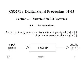
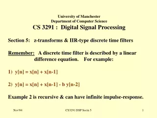
University of Manchester Department of Computer Science CS3291 Digital Signal Processing '05-'06 Section 4: ‘A design technique for FIR digital filters’. 4.1.Introduction:

E N D
University of Manchester Department of Computer Science CS3291 Digital Signal Processing '05-'06 Section 4: ‘A design technique for FIR digital filters’ CS3291: Section 4
4.1.Introduction: FIR digital filter of order M implemented by programming the signal flow graph shown below. Its difference equation is: y[n] = a0x[n] + a1x[n-1] + a2x[n-2] + ... + aMx[n-M] CS3291: Section 4
Its impulse-response is {..., 0, ..., a0, a1, a2,..., aM, 0, ...} • Its frequency-response is: • M • H(e j ) = a n e - j n • n=0 • Consider problem of choosing a0, a1,..., aM such that H( ej) is close to some target frequency-response. • Use the inverse DTFT: CS3291: Section 4
Assume we require low-pass filter whose gain-response approximates ideal 'brick-wall' gain-response:. If we take phase-response () = 0 for all , the required frequency-response is: CS3291: Section 4
By the inverse DTFT, = (1/3)sinc(n/3) for all n. CS3291: Section 4
sinc(x) 1 x -1 -3 -2 1 2 3 CS3291: Section 4
A digital filter with this impulse-response would have exactly the required low-pass frequency-response. • But {h[n]} has non-zero samples extending from n = - to , • Not a finite impulse-response. • Also not causal. CS3291: Section 4
To produce a realisable impulse-response: (1) Truncate {h[n]} to a FIR by setting h[n] to zero for all values of n outside the range -M/2 n M/2 ( assume M is the order of the required FIR filter and is even ). (2) Delay resulting sequence by M/2 samples to ensure that the first non-zero sample occurs at n = 0. CS3291: Section 4
M=10 n Starting with ideal impulse response: h[n] = (1/3)sinc(n/3) CS3291: Section 4
h[n] Truncate to M/2 M=10 n h[n] Delay by M/2 samples n CS3291: Section 4
Resulting causal impulse response realised by setting • an = h[n] for n=0,1,2,...,M. • Taking M=4, for example, the finite impulse response obtained for the /3 cut-off low-pass specification is : • {..,0,..,0, 0.14, 0.28, 0.33 , 0.28 , 0.14 , 0 ,..,0,..} CS3291: Section 4
x[n] z - 1 z - 1 z - 1 z - 1 0.14 0.28 0.33 0.28 0.14 y[n] • Resulting FIR filter is as shown below: • ( Note:4th order FIR filter has 4 delays & 5 multipliers ). • Gain & phase responses given in Figure 4.4. CS3291: Section 4
Fig 4.4 G(W} -f(W) dB -6 dB 0 -10 -20 W -30 W -p p/3 p p/3 p CS3291: Section 4
Truncating {h[n]} to M/2 & delaying by M/2 samples produces gain & phase responses different from those originally specified. • Gain-response: cut-off rate not sharp, • two "ripples" appear in stop-band, • peak of the first ripple at about -21dB. • Phase-response: not zero for all as orig specified, • ( ) = - ( M/2 ) for | | /3; • linear phase in pass-band • slope arctan(M/2) with M = 4 . • phase-delay M/2 = 2 samples. CS3291: Section 4
Question.Why does delaying {h[n]} by M/2 produce this effect? Answer: If DTFT of {h[n]} is H(ej) = G()ej(), the DTFT of the delayed impulse-response: Delaying {h[n]} by M/2 samples multiplies H(ej) by e-Mj/2 which increases () by -M / 2. Increases phase-delay -() / by M/2 sampling intervals. CS3291: Section 4
Can we improve low-pass filter by increasing order to ten? • Taking 11 terms of { (1 / n) sin (n / 3) } we get, • after delaying by 5 samples: • {...0,-0.055,-.069, 0,.138,.276,.333,.276,.138,0,-.069,-.055,0,...}. • If we analyse, by computer, a tenth order FIR filter with this impulse-response, we obtain the gain response shown in fig 4.5. CS3291: Section 4
The graph was produced by the following MATLAB statements: for n=1:11; a(n)= 0.3333*sinc((n-6)/3); end; H=freqz(a,1,1000); plot( [0:999]/1000, 20*log10(abs(H) ); axis( 0,1,-60,10] ); grid on; xlabel( ‘rel_freq / pi ); ylabel( ‘Gain (dB)’ ); Alternative graph may be produced by the single statement: freqz( [-0.055, -0.069, 0, 0.138, 0.276, 0.333, 0.276, 0.138, 0, -0.069, -0.055] ); CS3291: Section 4
A note on the phase-response graphs produced by ‘freqz’ • Plots () against rather than phase lag -(). • Segments at phase intervals of 2 or 360o () -() freqz 4 2 2 / 1 CS3291: Section 4
Gain response of 10th order lowpass FIR filter with WC = /3 CS3291: Section 4
Gain response of 20th order lowpass FIR filter with WC = /3 CS3291: Section 4
Cut-off rate for 10th order FIR filter sharper than for 4th order. • More stop-band ripples. • Gain at peak of first ripple after cut-off remains at -21 dB. • This effect is due to Gibb's phenomenon. • Linear phase in passband with phase delay of 5 samples. • Going to 20th order produces even faster cut-off rates, • & more stop-band ripples, • but main stop-band ripple remains at about -20dB. • To improve matters we need to discuss " windowing ". CS3291: Section 4
4.2. Windowing: To design FIR filters we multiplied {h[n]} as calculated by inverse DTFT by a rectangular window sequence {r[n]} where CS3291: Section 4
Causes sudden transition to zero at window edges. • It is these transitions that produce the stop-band ripples. • Levels of ripples reduced if {r[n]} replaced by non-rectangular window sequence { w[n] }. • Produces a more gradual transition at the window edges. • Simple non-rectangular window sequence is Hann window • It is a "raised cosine " CS3291: Section 4
Other types of window exist ( e.g. Hamming, Kaiser ). • Multiplying {h[n]} by {w[n]} instead of {r[n]} gradually tapers impulse-response towards zero at window edges. • Consider again low-pass filter example with rel cut-off /3. • Ideal impulse-response was found to be: • {h[n]} = { …..... , 0.14, 0.28, 0.33, 0.28, 0.14, ………} • When M = 4, the Hann window • {w[n]} = {..,0,..,0, 0.25, 0.75, 1, 0.75, 0.25, 0,..,0,..} • Multiplying term by term & delaying by M/2 = 2 samples we get: • {..,0,..,0, 0 .04, 0.21, 0.33, 0.21, 0.04, 0,..,0,..} CS3291: Section 4
x[n] z - 1 z - 1 z - 1 z - 1 a4 a3 a2 a0 a1 y[n] Resulting "Hann-windowed" FIR filter of order 4 is as shown below with a0=0.04, a1=0.21, a2=0.33, a3 = 0.21, a4 = 0.04. Its gain-response is approximately as shown in Figure 4.9. CS3291: Section 4
dB G(W) 0 -6dB -10 -20 -30 W p/3 2p/3 p Fig. 4.9 CS3291: Section 4
Figure 4.9: 4th order FIR filter (Hann) CS3291: Section 4
4.3 Effect of windowing on freq-response of FIR digital filter • Effect is to gradually reduce amplitude of ideal impulse-response towards zero at edges of window rather than to abruptly truncate. • Effect on gain-response of FIR filter obtained is: • i) to greatly reduce stop-band ripples ( good ). • ii) to reduce the cut-off rate ( bad ). • Phase-response is not affected in the pass-band. • We can improve the cut-off rate by going to higher orders. • Graphs below are for 10th & 20th order ( Hann windowed ): CS3291: Section 4
Tenth order FIR filter with C = /3 ( Hann window ) CS3291: Section 4
MATLAB program to design & graph 10th order FIR lowpass filter with Hann window w=hanning(11); for n=1:11; a(n) = 0.3333*sinc((n-6)/3)*w(n); end; h = freqz(a,1,1000); plot([0:999]/1000,20*log10(abs(h)),'k'); axis([0,1,-50,0]); grid on; xlabel('Rel_freq / pi'); ylabel('Gain(dB)'); CS3291: Section 4
20th order FIR filter with C = /3 (Hann window) CS3291: Section 4
4.4. Highpass, band-pass & band-stop linear phase FIR filters • Can be designed almost as easily as low-pass. • Remember to define required gain-response GI() from - to + • Make GI(-) = GI(). • Band-pass filter with pass-band from fS/8 to fS/4 has following gain response ideally:- CS3291: Section 4
Taking () = 0 for all initially as before, we obtain: • Applying the inverse DTFT (not forgetting negative ): • Can evaluate this, but there is a nicer way CS3291: Section 4
H(ej) = H1(ej) H2(ej) 1 1 -/2 - -/4 /4 - /2 = (1/2)sinc(n/2) - (1/4)sinc(n/4) for - < n < CS3291: Section 4
Exercise: By a similar method, or otherwise, show that the impulse-response for an ideal zero phase 'brick-wall' high-pass filter with cut-off frequency /6 radians per sample (i.e. one twelfth of the sampling frequency) is: h[n] = sinc(n) - (1/6)sinc(n/6) for - < n < Exercise: Derive the impulse-response for an ideal zero phase 'brick-wall' band-stop digital filter with cut-off frequencies L and U radians per sample. CS3291: Section 4
Technique not restricted to “conventional” gain-responses. • It is not difficult to design a linear phase filter whose gain-response approximates that below: CS3291: Section 4
4.5. Summary of design technique To design an FIR digital filter of even order M, with gain response G I () and linear phase by the windowing method, 1) Set H(ej) = G I () the required gain-response. This assumes () = 0. 2) IDTFT to produce the ideal impulse-response {h[n]}. 3) Window to M/2 using chosen window. 4) Delay windowed impulse-response by M/2 samples. 5) Realise by setting multipliers of FIR filter. CS3291: Section 4
Instead of obtaining H( ej) = G I ( ), we get e-jM/2G() • G() is distorted version of GI() due to windowing. • Phase-response is () = -M/2 which is linear phase . • -() / = M/2 for all . • Filter coeffs symmetric about M/2. • e.g. {…2, -3, 5, 7, 5, -3, 2, …} M =6 (even) • {…, 1, 3, 5, 5, 3, 1, …} M=5 (odd) • This is because the filters are linear phase. CS3291: Section 4
FIR digital filters whose impulse-responses are symmetric are linear phase. • Let {h[n]} = {…, 1, 3, 5, 5, 3, 1, …} • = e-5j/2 (e5j/2 +3e3j/2 +5ej/2 +5e-j/2 +3e-3j/2 +e-5j/2 ) • = e-5j/2 (2cos(2.5) + 6cos (1.5) + 10cos(/2) ) • = G()ej() with () = -5/2. • Hence () / = -5/2 = constant, so H(ej) is linear phase. CS3291: Section 4
Windowing or "Fourier series approxn technique ". • It is possible to design FIR filters which are not linear phase CS3291: Section 4
4.6 Further applications of windowing design technique • Technique even more powerful than has been yet indicated • Not restricted to linear phase filters. • Consider some further examples of its use. 4.6.1 Fractional sampling interval delay filter: 4.6.2. Differentiator: 4.5.3. Hilbert transformer: See notes for details CS3291: Section 4
4.6.1. Fractional sampling interval delay filter : Gain-response is one for all , but whose phase-response is () = - 0.5 . Therefore: e -j / 2 : 0 H(e j ) = e j / 2 : - 0 CS3291: Section 4
4.6.2. Differentiator: Would produce cos(t) from sin (t). FIR filter can act as a differentiator if it outputs {(/T) cos(n)} when the input is {sin(n)} for any in the range - to . Required gain-response is therefore G I () = /T. Instead of specifying a phase response of zero, specify a required phase lead of /2. Required frequency response is: (/T) e j / 2 : 0 j /T : 0 H(e j ) = = (/T e - j / 2 : - 0 -j /T : - 0 CS3291: Section 4
4.5.3. Hilbert transformer: G() = 1 and () = -/2 for 0 < < . “Quadrature phase” rather than linear phase. A linear phase component is added to the 90o phase shift when we delay the windowed impulse response for causality . The required frequency response is: e -j / 2 : 0 -j : 0 H(e j ) = 0 : = 0 = 0 : = 0 e j / 2 : - 0 j : - 0 CS3291: Section 4
Designing & implementing FIR digital filters using SP Toolbox • Design of linear phase FIR digital filters by windowing technique carried out by command 'FIR1'. • Applied to segment of sampled sound by command 'filter'. • Design & implement 128th order FIR band-pass digital filter with passband 300 Hz to 3.4 k Hz • Apply it to wav file of mono music sampled at 11.025 kHz. • Notes: • (1) FIR cut-off frequencies specified relative to fS/2 . • (2) By default FIR1 uses Hamming window; • (other windows such as Hann can be specified). • (3) Filter scaled so centre of pass-band has magnitude one. CS3291: Section 4
clear all; [x, fs, nbits] = wavread('caprice.wav'); %To design: wlow = 2 * pi * 300 / fs ; % radians/sample rel to fs wup = 2 * pi * 3400 / fs ; % radians/sample rel to fs a = fir1(128, [wlow wup] / pi ) ; freqz ( a , 1) ; % plot gain & phase % To implement: L=length(x); y = filter(a, 1, x ); % Remember the delay of 64 samples. wavwrite(x,fs,nbits,'capnew.wav'); CS3291: Section 4
Remez Exchange Algorithm method: • Better than windowing technique, but more complicated. • Available in MATLAB. • Design 40th order FIR lowpass filter whose gain is unity (0 dB) in range 0 to 0.3 radians/sample & zero in range 0.4 to . • The 41 coefficients will be found in array ‘a’. • Produces 'equi-ripple' gain-responses where peaks of stop-band ripples are equal rather than decreasing with increasing frequency. • Highest peak in stop-band lower than for FIR filter of same order designed by windowing technique to have same cut-off rate. • There are 'equi-ripple' pass-band ripples. CS3291: Section 4
a = remez (40, [0, 0.3, 0.4,1],[1, 1, 0, 0] ); h = freqz (a,1,1000); plot([0:999]/1000,20*log10(abs(h)),'k'); axis([0,1,-50,0]); grid on; xlabel('Rel_freq / pi'); ylabel('Gain(dB)'); CS3291: Section 4
Gain of 40th order FIR lowpass filter designed by “ Remez ” CS3291: Section 4
4.9. Some implementation issues • 4.9.1. Fixed point implementation of FIR digital filters • FIR digital filters often implemented in mobile equipment. • Low power fixed point DSP processors are norm. • Typically with a basic 16-bit word-length. • Must be programmed using only integer arithmetic. • Take 4th order FIR filter with impulse response: • {….. 0.04, 0.21, 0.33, 0.21, 0.04, …...}. • Rounding each coeff to nearest integer clearly a mistake. • Multiply all coeffs by a large constant then round: . • A0 = 4, A1 = 21, A2 = 33, A3 = 21 , A4 = 4. • We must divide the output by same constant, in this case 100. • Instead of 100, we choose a power of two for the constant. • Dividing by a power of two (e.g. 1024) is very simple. CS3291: Section 4