Download
1 / 29
300 likes | 704 Vues
CHAPTER 16 Standard Deviation of a Discrete Random Variable. First center (expected value) Now - spread. Standard Deviation of a Discrete Random Variable. Measures how “spread out” the random variable is. Data Histogram measure of the center: sample mean x measure of spread:

E N D
CHAPTER 16Standard Deviation of a Discrete Random Variable First center (expected value) Now - spread
Standard Deviation of a Discrete Random Variable Measures how “spread out” the random variable is
Data Histogram measure of the center: sample mean x measure of spread: sample standard deviation s Random variable Probability Histogram measure of the center: population mean m measure of spread: population standard deviation s Summarizing data and probability
Example • x 0 100 p(x) 1/2 1/2 E(x) = 0(1/2) + 100(1/2) = 50 • y 49 51 p(y) 1/2 1/2 E(y) = 49(1/2) + 51(1/2) = 50
Variation The deviations of the outcomes from the mean of the probability distribution xi - µ 2 (sigma squared) is the variance of the probability distribution
Economic Scenario Profit ($ Millions) Probability X P Great 10 0.20 x1 P(X=x1) 5 Good 0.40 x2 P(X=x2) OK 1 0.25 x3 P(X=x3) Lousy -4 0.15 x4 P(X=x4) Variation Example 2 = (x1-µ)2 · P(X=x1) + (x2-µ)2 · P(X=x2) + (x3-µ)2 · P(X=x3) + (x4-µ)2 · P(X=x4) = (10-3.65)2 · 0.20 + (5-3.65)2 · 0.40 + (1-3.65)2 · 0.25 + (-4-3.65)2 · 0.15 = 19.3275 3.65 3.65 3.65 3.65 P. 207, Handout 4.1, P. 4
2 = 19.3275 Standard Deviation , or SD, is the standard deviation of the probability distribution
Probability Histogram = 4.40 µ=3.65
Finance and Investment Interpretation • X = return on an investment (stock, portfolio, etc.) • E(x) = m = expected return on this investment • sis a measure of the risk of the investment
Example (cont.) m=1.5, s=.866 • Specify the interval (m - 1s, m + 1s) • (1.5 - 1(.866), 1.5 + 1(.866)) (1.5 - .866, 1.5 + .866) (.634, 2.366) • P(.634 x 2.366) = • p(1)+p(2)=3/8 + 3/8 = 3/4
68-95-99.7 Rule for Random Variables For random variables x whose probability histograms are approximately mound-shaped: • P(m - s x m + s) .68 • P(m - 2s x m + 2s) .95 • P(m -3s x m + 3s) .997
Rules for E(X), Var(X) and SD(X):adding a constant a • If X is a rv and a is a constant: • E(X+a) = E(X)+a • Example: a = -1 • E(X+a)=E(X-1)=E(X)-1
Rules for E(X), Var(X) and SD(X): adding constant a (cont.) • Var(X+a) = Var(X) SD(X+a) = SD(X) • Example: a = -1 • Var(X+a)=Var(X-1)=Var(X) • SD(X+a)=SD(X-1)=SD(X)
Economic Scenario Profit ($ Millions) X Probability Economic Scenario Profit ($ Millions) X+2 Probability P P Great 10 0.20 Great 10+2 0.20 x1 x1+2 P(X=x1) P(X=x1) 5 5+2 Good 0.40 Good 0.40 x2 x2+2 P(X=x2) P(X=x2) OK 1 0.25 OK 1+2 0.25 x3 x3+2 P(X=x3) P(X=x3) Lousy -4 0.15 Lousy -4+2 0.15 x4 x4+2 P(X=x4) P(X=x4) E(x + a) = E(x) + a; Var(x + a)=Var (x); let a = 2 = 4.40 = 4.40 m=5.65 m=3.65
New Expected Value Long (UNC-CH) way: E(x+2)=12(.20)+7(.40)+3(.25)+(-2)(.15) = 5.65 Smart (NCSU) way: a=2; E(x+2) =E(x) + 2 = 3.65 + 2 = 5.65
New Variance and SD Long (UNC-CH) way: (compute from “scratch”) Var(X+2)=(12-5.65)2(0.20)+… +(-2+5.65)2(0.15) = 19.3275 SD(X+2) = √19.3275 = 4.40 Smart (NCSU) way: Var(X+2) = Var(X) = 19.3275 SD(X+2) = SD(X) = 4.40
Rules for E(X), Var(X) and SD(X): multiplying by constant b • E(bX)=b E(X) • Var(b X) = b2Var(X) • SD(bX)= |b|SD(X) • Example: b =-1 • E(bX)=E(-X)=-E(X) • Var(bX)=Var(-1X)= =(-1)2Var(X)=Var(X) • SD(bX)=SD(-1X)= =|-1|SD(X)=SD(X)
Expected Value and SD of Linear Transformation a + bx Let X=number of repairs a new computer needs each year. Suppose E(X)= 0.20 and SD(X)=0.55 The service contract for the computer offers unlimited repairs for $100 per year plus a $25 service charge for each repair. What are the mean and standard deviation of the yearly cost of the service contract? Cost = $100 + $25X E(cost) = E($100+$25X)=$100+$25E(X)=$100+$25*0.20= = $100+$5=$105 SD(cost)=SD($100+$25X)=SD($25X)=$25*SD(X)=$25*0.55= =$13.75
Addition and Subtraction Rules for Random Variables • E(X+Y) = E(X) + E(Y); • E(X-Y) = E(X) - E(Y) • When X and Y are independent random variables: • Var(X+Y)=Var(X)+Var(Y) • SD(X+Y)= SD’s do not add: SD(X+Y)≠ SD(X)+SD(Y) • Var(X−Y)=Var(X)+Var(Y) • SD(X −Y)= SD’s do not subtract: SD(X−Y)≠ SD(X)−SD(Y) SD(X−Y)≠ SD(X)+SD(Y)
In general, if X and Y are RVs, Var(X+Y) ≠ Var(X)+Var(Y) SD(X+Y) ≠ SD(X)+SD(Y) Special case (previous slide): If RVs are Independent: Variances add: Var(X+Y)=Var(X)+Var(Y) but… Standard Deviations still DO NOT add: SD(X+Y)≠SD(X)+SD(Y)
Pythagorean Theorem of Statistics: variances add; standard deviations do not add a2 + b2 = c2 Var(X)+Var(Y)=Var(X+Y) c2 Var(X) Var(X+Y) c a2 a SD(X+Y) SD(X) a + b ≠ c SD(X)+SD(Y) ≠SD(X+Y) b SD(Y) b2 Var(Y)
Pythagorean Theorem of Statistics: variances add; standard deviations do not add 32 + 42 = 52 Var(X)+Var(Y)=Var(X+Y) 25 Var(X) Var(X+Y) 5 9 3 SD(X+Y) SD(X) 3 + 4 ≠ 5 SD(X)+SD(Y) ≠SD(X+Y) 4 SD(Y) 16 Var(Y)
Motivation forVar(X-Y)=Var(X)+Var(Y) • Let X=amount automatic dispensing machine puts into your 16 oz drink (say at McD’s) • A thirsty, broke friend shows up. Let Y=amount you pour into friend’s 8 oz cup • Let Z = amount left in your cup; Z = ? • Z = X-Y • Var(Z) = Var(X-Y) = Var(X) Has 2 components + Var(Y)
For random variables, X+X≠2X • Let X be the annual payout on a life insurance policy. From mortality tables E(X)=$200 and SD(X)=$3,867. If the payout amounts are doubled, what are the new expected value and standard deviation? • Double payout is 2X. E(2X)=2E(X)=2*$200=$400 • SD(2X)=2SD(X)=2*$3,867=$7,734 • Suppose insurance policies are sold to 2 people. The annual payouts are X1 and X2. Assume the 2 people behave independently. What are the expected value and standard deviation of the total payout? • E(X1 + X2)=E(X1) + E(X2) = $200 + $200 = $400 The risk to the insurance co. when doubling the payout (2X) is not the same as the risk when selling policies to 2 people.