Download
1 / 63
630 likes | 648 Vues
This paper explores the adaptation of dendritic spines shape using a genetic algorithm. The study involves the geometrical reconstruction of dendritic spines and simulation experiments on different morphologies.

E N D
Adaptation of shape of dendritic spines by genetic algorithm A. Herzog1, V. Spravedlyvyy1, K. Kube1, E. Korkotian3, K. Braun2, B. Michaelis1 1 Institute of Electronics, Signal Processing and Communications, 2 Institute of Biology; Otto-von-Guericke University Magdeburg, P.O.Box 4120, 39016 Magdeburg, Germany 3 The Weizmann Institute, Department of Neurobiology, Rehovot 76100, Israel
5 number of spine 4 3 2 1 0 0.02 0.04 0.06 0.08 0.1 simulation time in [s] Overview 1 Geometrical reconstruction of dendritic spines 3D Confocal Image Geometric Model 2 Simulation experiments on different morphology
Introduction I Nerve cell, biological background Input from other nerve cells Synapses Dendrites passive transmission Soma impulse coding Active impulse transmission Axon Output to other nerve cells
Introduction II dendrites 2 µm dendritic spines • Dendritic spines • type of input terminal • signal transmission modulated by size and shapemorphological studies: • spines changes during learning • and development • Image processing • measure size and shape of spines to underlay biol. experiments • experimental and control group • statistic significant: thousands of spines need dendritic tree with spines
Image Acquisition confocal laser-scanning microscope (CLSM) 3D-scanning nerve cell filled by fluorochrome dye real 3D image (stack) Bead (1µm) • advantage: • resolution good enough • fast (statistics need many images) • disadvantage: • an-isotropic PSF (point spread function) • deconvolution is need but limited by noise xy xz
Direction depend sharpness Shape changes in image Object size, graylevel Original Bead (1µm) Convolved by PSF xy - Projection small objects => Smaller graylevel PSF (turned) xz - Projection Influence of Point-spread function Correction is necessary
circular Cross section Chain model by model points radius Reconstruction by geometric model Geometric model of spine Piece wise linear Approximation by centre axis and local radius • only few voxel • un sharp • not enough to get position of border • simplifications Also use for dendrite reconstruction
Connection of base elements Model element • 2 points • 2 radiuses chain Chain with branching Connect by “Constructive Solid Geometry”
Estimation of model parameters in two steps 1st step Rough model of centre axis of dendrite and all spines Interactive correction 2dt step Accurate estimation of model parameters, microscope PSF taken into account • Benefit • all visible spines include • lower subjective influence as • draw model border directly
Find centre axis by growing model Basic idea: • place first element(s) interactively (initialisation) • following elements set automatically • element size fixed, estimate direction • Estimate of direction: • test several direction (ca. 100) • rate direction in respect to a-priori knowledge
criteria average graylevel in ROI ROI Fuzzy or ANN Local change of direction tested direction Global change of direction quality of direction Tested direction Rate quality of direction A-priori combine graylevel inside object is higher No fast change of direction Follow main Direction (no loops) Follow direction of highest quality (including constrains)
Branching offs • test all model points • new locale criteria: orthogonal to centre axis test direction Special cases Branching off of spine • found hull around dendrite • get local peaks of graylevel • connection to dendrite • growing up to spine head
Smoothing and adapting of centre axis Smoothing Check average graylevel on alternative (shorter) route Adjust axis • centre of mass in ROI • move model point in orthogonal plane to centre axis • to it several times
Result of model growing Part of dendrite with spines Dendrite tree • Summery • no complicated pre-processing (deconvolution) is need • include all visible spines by interaction
1st step Rough model of centre axis of dendrite and all spines Estimation of model parameters in two steps Interactive correction 2dt step High quality estimation of Model parameters, microscope PSF taken into account
Iterative estimation of parameters geometric model Initialisation Convert in 3D-image Optimisation of Model parameters Simulation of microscope imaging convolution by PSF constrains • position relations • shape • size microscope- image Compare Error function:
Octree-Model outside Octree Model inside On border splitting splitting Subvoxel Subvoxel Voxel binary operation to overlap elements available
Iteration, gradient decent: Step size direction Numeric calculation of gradient Very high numerical consumptions (simulation of microscope imaging) Estimate gradient by a simplermodel Optimisation of model parameters
Points with mass Direct method (concentrated parameter) Model Microscope image If model inside a ROI small in relation to PSF => specific shape of model does no matter • simplification • model of mass points
Image point PSF Direct method (concentrated parameter) • Graylevel of a image point • Superposition of parts of all mass points All points in ROI Model Microscope image For all points inside ROI Result: Mass of ROI i coefficient (PSF, ROI)
Linear equation system For all ROI coefficient coefficients (Bandmatrix) Mass of ROI in Microscope image Points mass • get mass of ROI in microscope image • solve equation system • convert point mass to cylinder with sufficient radius
Radius in Voxel 2 result target 1 0 8 12 16 4 0 Model point Results of direct method Simulated spine Real spine Maxium projection Shadow projection Geometric model
Position of model points Vector between centre of mass Estimation of gradients Local radius Difference of mass real microscope image vs. simulated image coefficient Length of ROI Rotation symmetry is only an asummtion • controll error • change radius and position alternativly • reduce step size
Error (average graylevel) 12 8 4 0 10 20 30 40 0 Iteration Result (artificial spine) Simulated microscope image Model 15 radiuses Estimated gradient speeds up 15 times
Result (real spine) Radius (voxel size) direct method 6.2 2 numeric gradient konzentrierte Parameter 4,2 Iteration 1 (numerisch) Iteration 2 (geschätzt) estimated gradient 1 4,45 0 4 12 8 MSE (all ROI) Model point
Parameters from geometric model rel. number iso-group 0.2 soc-group 0.1 0 0 volume [µm³] 5 10 15 20 • Geometric parameter • length, diameter • volume • axes, moments • head, neck • position, density ... Spines with different size and shape • Functional parameters ? • electric simulation need volume ( 3000 Spines)
Electrical simulation of spine behaviour input-spike head simulation by „genesis“ base Schematic spine • Electrical simulation • compartment model • glutamate synapse 4 ms • single spike response • main interest PSP on spine base
Compartment 2 3 4 5 Spine 1 dh head lh ln neck R distal a dn C proximal base dendrite m R m spine position dendrite + soma 2,5 µm Electrical Simulation • Compartment model • split into coupled compartments: 3 head, 7 neck, 20 dendrite • special compartment (dendrite + soma) • differential equations numeric solved by “genesis” • Simplify geometry • 4 basic geometric parameters per spine: dh , lh dn ln • 5 Spines • all other parameters fixed
asynchronous spikes synchronous spikes 5 5 4 4 number of spine number of spine 3 3 2 2 1 1 0 0.02 0.04 0.06 0.08 0.1 0 0.02 0.04 0.06 0.08 0.1 simulation time in [s] simulation time in [s] Information processing in groups of Spines Idea: adapt geometry to better distinguish different signals Distinguish different synchronicity • Genetic algorithm + Simulated annealing • 20 genes (5 spines; 2 length, 2 diameter per spine • 50 individuals (2 elitist) • 1 GA => 10 SA steps • change spine position
-3 x 10 best individual 9 8 worst individual 7 average fitness 6 5 4 generation 400 fitness = 0.008427 generation 1 fitness = 0.006955 generation 200 fitness = 0.008352 3 2 0 50 100 150 200 250 300 350 400 generation Results Synchronous, asynchronous
asynchronous spikes synchronous spikes 5 5 4 4 number of spine number of spine 3 3 2 2 1 1 0 0.02 0.04 0.06 0.08 0.1 0 0.02 0.04 0.06 0.08 0.1 simulation time in [s] simulation time in [s] PSP postsynaptic potential (PSP) 0.03 0.03 0.025 0.025 membran potential [mV] 0.02 0.02 membran potential [mV] 0.015 0.015 0.01 0.01 0.005 0.005 0 0 0 0.02 0.04 0.06 0.08 0.1 0 0.02 0.04 0.06 0.08 0.1 simulation time in [s] simulation time in [s] Results
5 number of spine 4 3 2 1 0 0.02 0.04 0.06 0.08 0.1 simulation time in [s] 0.03 0.03 0.025 0.025 0.02 membran potential [mV] 0.02 0.015 0.015 0.01 0.01 0.005 0.005 0 0 0.02 0.04 0.06 0.08 0.1 0 simulation time in [s] 0 0.02 0.04 0.06 0.08 0.1 simulation time in [s] Sequence and backward sequence Sequence Backward Sequence 5 number of spine 4 3 2 1 0 0.02 0.04 0.06 0.08 0.1 simulation time in [s] postsynaptic potential (PSP) postsynaptic potential (PSP) membran potential [mV]
-3 x 10 6 4 fitness 2 0 -2 -4 0 50 100 150 200 250 generation Results II
600 z [µm] 400 200 0 600 100 400 50 200 y [µm] x [µm] 0 0 - 50 Future work • Spine on dendrite • statistic parameters • (distribution of size, • shape, clustering) • dendrite (statistical) parameters Growing dendrite by statistic parameters
Conclusion • Image processing • high quality model confocal images • statistics for geometrical parameters • Simulation experiments • idea: change geometry to learn new behaviour • small group of five spines • distinguish different signal timings by adapting geometry by genetic algorithm
Scanning mirror Beam splitter y Laser x Pin holes lenses photo multiplier z Probe Nerve cell, filled by dye Confocal laser scanning microscope (CLSM)
Original image Deconvolution Result of deconvolution
Geometrical reconstruction of dendritic spines Form 3d image to geometrical model Geometric Model 3D Confocal Image (shadow projection)
Simulation of microscope imaging Sample model Convolution by PSF
Distance Centre voxel to model inside, neg. value Octree-Model, Cases 0 1 Cases 2 3 4 Smallest splitting => linear interpolation
geometric model simulated imaging by microscope Simulated Microscope image Object function (distribution of dye) Imaging by microscope real Microscope image Higher quality estimation of model parameters including PSF Compare • Two methods • direct method by simplified model • iterative method
Electrical Simulation Simulation experiments on dendritic spines with variable geometry • Introduction • dendritic spines • motivation • Geometrical reconstruction of dendritic spines - Image processing • Electrical simulation of functional spines • Learning by geometrical changes • Genetic algorithm
membrane Compartment model
Peak of PSP, V length of neck, µm diameter of neck, µm Variation of single spine • Geometric Variation • four geometric parameter • 10 steps each • 10.000 test • Measured values • peak potential • area • delay • Parallel Processing • Linux-Cluster “Minerva” • 32 nodes (64 processors) • app. 2 h (10.000 variations) Peak potential [ESAN]
V V V - 0.07 - 0.07 - 0.07 t t t Characteristic Values Compare results ? • Delay • coincidence detection • sequence distinguish • Area • energy impact • background level • Peak potential • nonlinear behavior • local action potential in dendrite Position of spine ? • Note • no synapse dynamics !
Delay, sec Peak of PSP, V length of neck, µm length of neck, µm diameter of neck, µm diameter of neck, µm Systematic variations Peak potential Delay • Diagrams • 10.000 sample points in 4 dimensions • every slice represent different head geometry • restrictions dh > dn