Download

1 / 29
320 likes | 751 Vues
Hydrodynamic Slip Boundary Condition for the Moving Contact Line. in collaboration with Xiao-Ping Wang ( Mathematics Dept, HKUST ) Ping Sheng ( Physics Dept, HKUST ). ?. No-Slip Boundary Condition. from Navier Boundary Condition to No-Slip Boundary Condition.

E N D
Hydrodynamic Slip Boundary Condition for the Moving Contact Line in collaboration with Xiao-Ping Wang (Mathematics Dept, HKUST) Ping Sheng (Physics Dept, HKUST)
? No-SlipBoundary Condition
from Navier Boundary Conditionto No-SlipBoundary Condition : shear rate at solid surface : slip length, from nano- to micrometer Practically, no slip in macroscopic flows
No-SlipBoundary Condition ? Apparent Violation seen from the moving/slipping contact line Infinite Energy Dissipation (unphysical singularity) Are you able to drink coffee?
Previous Ad-hoc models:No-slip B.C.breaks down • Nature of the true B.C. ? (microscopic slipping mechanism) • If slip occurs within a length scale Sin the vicinity of the contact line, then what is the magnitude of S ?
Molecular Dynamics Simulations • initial state: positions and velocities • interaction potentials: accelerations • time integration: microscopic trajectories • equilibration (if necessary) • measurement: to extract various continuum, hydrodynamic properties • CONTINUUM DEDUCTION
Molecular dynamics simulationsfor two-phase Couette flow • Fluid-fluid molecular interactions • Wall-fluid molecular interactions • Densities (liquid) • Solid wall structure (fcc) • Temperature • System size • Speed of the moving walls
Modified Lennard-Jones Potentials for likemolecules for molecules of different species for wetting property of the fluid
fluid-2 fluid-1 fluid-1 dynamic configuration f-1 f-2 f-1 f-1 f-2 f-1 symmetric asymmetric static configurations
boundary layer tangential momentum transport
The Generalized NavierB. C. when the BL thickness shrinks down to 0 viscous part non-viscous part Origin?
uncompensated Young stress nonviscous part viscous part
Uncompensated Young Stressmissed in Navier B. C. • Net force due to hydrodynamic deviation from static force balance (Young’s equation) • NBCNOTcapable of describing the motion of contact line • Away from the CL, the GNBC implies NBCfor single phase flows.
Continuum Hydrodynamic ModelingComponents: • Cahn-Hilliard free energy functional retains the integrity of the interface(Ginzburg-Landau type) • Convection-diffusion equation (conserved order parameter) • Navier - Stokes equation(momentum transport) • Generalized Navier Boudary Condition
Diffuse Fluid-Fluid Interface Cahn-Hilliard free energy (1958)
capillary force density is the chemical potential.
= tangential viscous stress + uncompensated Young stress Young’s equation recovered in the static case by integration along x
for boundary relaxation dynamics first-order generalization from in equilibrium, together with
Comparison of MD and Continuum Hydrodynamics Results • Most parameters determined from MDdirectly • M and optimized in fitting the MD results for one configuration • All subsequent comparisons are without adjustable parameters.
near-total slipat moving CL SymmetricCoutte V=0.25 H=13.6 no slip
profiles at different z levels symmetric Coutte V=0.25 H=13.6 asymmetricCoutte V=0.20 H=13.6
symmetricCoutte V=0.25 H=10.2 symmetricCoutte V=0.275 H=13.6
The boundary conditions and the parameter values are bothlocal properties, applicable to flows with different macroscopic/external conditions (wall speed, system size, flow type).
Summary: • A need of the correct B.C. for moving CL. • MD simulations for the deduction of BC. • Local, continuum hydrodynamics formulated from Cahn-Hilliard free energy, GNBC, plus general considerations. • “Material constants” determined (measured) from MD. • Comparisons between MD and continuum results show the validity of GNBC.
Large-Scale Simulations • MD simulations are limited by size and velocity. • Continuum hydrodynamic calculations can be performed with adaptive mesh (multi-scale computation by Xiao-Ping Wang). • Moving contact-line hydrodynamics is multi-scale (interfacial thickness, slip length, and external confinement length scale).