Download
1 / 37
400 likes | 521 Vues
Explore simulation results, error analysis & operation modes of SPL's RF cavities using MATLAB Simulink. Understand beam loading, feedback loop, and Lorentz effects.

E N D
LLRF Cavity Simulation for SPL Simulink Model for HP-SPL Extension to LINAC4 at CERN from RF Point of View Acknowledgement: CEA team, in particular O. Piquet (simulink model) W. Hofle, J. Tuckmantel, D. Valuch, G. Kotzian, F. Gerigk, M. Schuh, P. A. Posocco
Presentation Overview • SPL Characteristics • Single Cavity Model and Simulation Results • Dual Cavity Model and Simulation Results • Error Analysis
SPL High Current Operation • Possible operation using 1, 2 and 4 cavities fed by a single power amplifier. 1 Cavity per Klystron 2 Cavities per Klystron
RF Drive and Generator Model • Generator current modeled as square pulse for the duration of injection + beam pulse time • High bandwidth compared to feedback loop and cavity (1 MHz)
Cavity Model (cont) Simplified Diagram Cavity differential equations, generator plus beam loading voltage gradients result in output curve for cavity voltage envelope.
Beam Loading • Infinitely narrow bunches induce instant voltage drops in cavity • Voltage drop is equal to generator induced voltage increase between bunches creating flattop operation • Envelope of RF signal in I/Q
RF Feedback • PID controller • Limit bandwidth in feedback loop to 100 kHz • (Klystron bandwidth is 1 MHz) “soft” switch possibility for transient reduction
Results • Cavity Voltage Amplitude and Phase • Forward and Reflected Power • Additional Power for Feedback Transients and Control • Effect of Lorentz Detuning on Feedback Power • Effect of Source Current Fluctuations • Mismatched Low-Power Case • Effects of Beam Relativistic Beta Factor on Cavity Voltage During Beamloading
Cavity Voltage Magnitude and Phase in the Absence of Lorentz Detuning (Open Loop) Reactive Beamloading Results in Vacc Deviation Phase Displayed Between Generator and Cavity
Effect of Lorentz Detuning on Cavity Voltage and Phase(Lorentz Frequency Shift)
Effect of Lorentz Detuning on Cavity Voltage and Phase (Open Loop) Lorentz effects oppose those of the synchronous angle Approximately linear phase shift for undriven cavity during field decay
Effect of Lorentz Detuning on Cavity Voltage and Phase (Open Loop Close-Up) Negative Lorentz detuning factor has opposite effect on cavity voltage magnitude with respect to synchronous angle effects. Negative Lorentz detuning factor has opposite effect on phase with respect to synchronous angle effects.
Cavity Voltage and Phase With Lorentz Detuning(Closed Loop Performance of Fast Feedback)
Cavity Voltage and Phase Close-up Injection Time (start of beam pulse)
Forward and Reflected Power without Lorentz Detuning Feedback loop is closed (ON) 10 us after start of generator pulse and opened (OFF)10 us after end of the beam pulse.
Forward and Reflected Power with Lorentz Force detuning Less power is necessary to maintain cavity voltage due to opposing effects of synchronous angle and Lorentz detuning Feedback loop is closed 10 us after start of generator pulse and opened 10 us after the end of the beam pulse.
Effects of Source Beam Current Variation 5% variation in Ib for 40mA case requires approximately 60kW of additionalpower.
SPL Low Current Operation (Power Analysis) QLmismatch before beamloading
Effects of Source Beam Current Variation 5% (1mA) results in approx. 20kW FB power increase
Transit Time Factor Variation with Relativistic Beta (SPL β=1 cavities) • The shunt impedance relates the voltage in the cavity gap to the power dissipated in the cavity walls. • The corrected shunt impedance (effective shunt impedance) relates the accelerating voltage in the cavity to the power dissipated. This quantity describes the voltage that a particle travelling at a certain speed will “see” when traversing the cavity. • The correction applied is known as the “Transit Time Factor”. For even symmetric field distributions:
Transit Time Factor Variation with Relativistic Beta (SPL β=1 cavities) • Until now, the cavity dynamics have been modeled from the point of view of a beam travelling at the speed of light (β =1). • We now investigate how the cavity voltage is affected during beam loading with a “slower” beam.
Transit Time Factor Variation with Relativistic Beta (SPL β=1 cavities, open loop simulation) Beamloading Values obtained from SUPERFISH simulations by Marcel Schuh (CERN) Beamloading • Weaker beamloadingwill result in a higher flattop equilibrium and less phase detuning of the cavity for the same generator power. • Beta value taken from beam energy at beginning of SPL β=1 section.
Results • Cavity Phase Variation Without Feed-Forward • Effects of Adaptive Feed-Forward • Effects of Loaded Quality Factor Variation
Vcav Magnitude and Phase for Dual Cavity Case(K=-1 and -0.5) Voltage magnitude and phase of vector average
Vcav Magnitude and Phase for Dual Cavity Case(Without Feed-Forward) K=-0.5 K=-1
Vcav Magnitude and Phase for Dual Cavity Case(With Feed-Forward) Cavity 1 (K=-1 ) Cavity 2 (K=-0.5 )
Loaded Quality Factor Fluctuation Effects on Cavity Voltage Magnitude Ql2-Ql1=20000 Ql2-Ql1=30000 +-0.5% +-0.5% +-0.5% +-0.5%
Error Analysis • Vector average is maintained within specifications with RF feedback loop, but individual cavities deviate depending on their parameters. • Characterize deviation of cavity voltage with variations in loaded quality factor and Lorentz detuning coefficients • Curves fitted for difference in cavity voltage magnitude and phase between 2 cavities controlled by a single RF feedback loop, with a setpointat nominal accelerating voltage magnitude and phase. • With this information, the overall effects of the cavity voltage deviation due to Lorentz detuning and loaded quality factor mismatches can be investigated with a model for the whole length of the SPL (investigated at CERN by Piero Antonio Posocco).
Effects of Varying Loaded Quality Factor on Cavity Voltage Magnitude p00=1.725e+006 p10=34.88 p01=-37.66 p20=-8.311e-006 p11=1.527e-007 p02=9.27e-006
Effects of Varying Lorentz Detuning Coefficient on Cavity Voltage Magnitude p00= 25.8 p10= -2.05e+014 p01= 2.014e+014 p20= -3.496e+028 p11= -1.565e+026 p02= 3.505e+028
Effects of Varying Lorentz Detuning Coefficient on Cavity Voltage Phase p00= -0.0004408 p10= 3.768e+012 p01= -3.768e+012
In Summary… • In order to cater for the needs of project specifications, a high flexibility simulation model was developed. • Flexible graphical user interface allows for efficient handling of simulation data. • 1, 2 and 4 cavities can be observed from RF point of view for a wide set of parameters. • Can estimate practical issues that can arise during development of the real LLRF system in terms of power, stability of accelerating field and technology necessary for operation.
Next Step • Investigate different possible optimisationsto transit time factor effects in terms of forward power, loaded quality factor and injection time along the LINAC. • Characterize power amplifier and other components from real measurements in terms of their transfer functions. • Characterize the behavior of the piezo-electronic tuner within the control loop. • Develop a full digital/analogue control system using hardware and test in a cold cavity.