Download
1 / 40
410 likes | 668 Vues
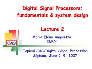
Digital Signal Processors: fundamentals & system design Lecture 2. Maria Elena Angoletta CERN. Topical CAS/Digital Signal Processing Sigtuna, June 1-9, 2007. Lectures plan. Lecture 1. introduction, evolution, DSP core + peripherals. Lecture 2.

E N D
Digital Signal Processors: fundamentals & system design Lecture 2 Maria Elena Angoletta CERN Topical CAS/Digital Signal Processing Sigtuna, June 1-9, 2007
Lectures plan Lecture 1 introduction, evolution, DSP core + peripherals Lecture 2 DSP peripherals (cont’d), s/w dev’pment & debug. Lecture 3 System optimisation, design & integration. M. E. Angoletta, “DSP fundamentals & system design – LECTURE 2”, CAS 2007, Sigtuna 2/40
Lecture 2 - outline Chapter 4 DSP peripherals (cont’d) Chapter 5 RT design flow: introduction Chapter6 RT design flow: s/w development Chapter7 RT design flow: debugging M. E. Angoletta, “DSP fundamentals & system design – LECTURE 2”, CAS 2007, Sigtuna 3/40
Chapter 4 topics DSP peripherals 4.1 Introduction 4.2 Interconnect & I/O 4.3 Services 4.4 C6713 example 4.5 Memory interfacing 4.6 Data converter interfacing 4.7 DSP booting Summary Yesterday Now M. E. Angoletta, “DSP fundamentals & system design – LECTURE 2”, CAS 2007, Sigtuna 4/40
4.5 Memory interfacing • H/w interface often available in TI & ADI DSPs. Ex: TI External Memory InterFace (EMIF). • Glueless interface to SRAM, EPROM, Flash, SBSRAM, SDRAM. C6713: 32-bit EMIF, 512 MByte addressable ext. memory space. • No dedicated h/w interface → external h/w (ex: FPGA). • Synchronous or asynchronous interface (DSP-driven). • Address decoding. • Careful with priority & interleaved memory access (data integrity). Ex: ADI SHARC. Generic DSP-external memory interfacing scheme. M. E. Angoletta, “DSP fundamentals & system design – LECTURE 2”, CAS 2007, Sigtuna 5/40
4.6 Data converters interfacing • TI: Serial interfaces McBSP, McASP +DMA. • Also EMIF in asynchronous mode + DMA. • ADI: Parallel Peripheral Interface (PPI) on Blackfin . • Bidirectional data flow + Serial Port Interface (SPI) to init/configure converter. ADSP-BF533 Blackfin to AD9975 mixed-signal modem front-end interface. • General solution: FPGA to rebuffer/pre-process (ex.: filtering) data. • Mixed-signal DSPs: on-board ADC/DAC. EX: ADSP-21190 M. E. Angoletta, “DSP fundamentals & system design – LECTURE 2”, CAS 2007, Sigtuna 6/40
4.7 DSP booting POWER IN • Debugging: executable files uploaded to DSP via JTAG. • Exploitation: DSP boots without JTAG. • Booting mode defined by DSP input pins. • Methods: • No-boot: DSP fetches instructions directly from EPROM/FLASH. • ROM boot: DSP reads formatted boot stream from ROM. • Host boot: DSP stalled until host configures memory. TI ‘C6x DSP booting from ROM. M. E. Angoletta, “DSP fundamentals & system design – LECTURE 2”, CAS 2007, Sigtuna 7/40
Chapter 4 summary • Peripherals: wide range & important parameters for DSP choice. • Interconnect & data I/O: serial + parallel interfaces. • Services: PLL, timers, JTAG, power management… • Memory interfaces • Dedicated: ex. TI EMIF • FPGA: DSP-driven synchronous/asynchronous • Data converters interfaces • Serial or parallel • JTAG • Load code / debug • For exploitation DSP boots from memory. M. E. Angoletta, “DSP fundamentals & system design – LECTURE 2”, CAS 2007, Sigtuna 8/40
5. RT design flow: introduction • Defines • architecture • interfaces • data flow • control • Debugs • Simulation • Emulation • System integration • within controls infrastructure • Develops • s/w project(s) • code • config. file • Analyse & optimise • Evaluate performance • Optimise selected parts M. E. Angoletta, “DSP fundamentals & system design – LECTURE 2”, CAS 2007, Sigtuna 9/40
Chapter 6 topics RT design flow: s/w development 6.1 DSP programming – intro. 6.2 Development setup + environment. 6.3 Languages: assembly, C, C++, graphical. 6.4 RTOS. 6.5 Code building process. Summary M. E. Angoletta, “DSP fundamentals & system design – LECTURE 2”, CAS 2007, Sigtuna 10/40
6.1 DSP programming - intro • DSPs: programmed by software. • Languages: • High-level software tools (ex. MATLAB, National Instruments … ) to automatically generate files. → Rapid prototyping! • Cross-compilation: code developed & compiled on different machine (PC, SUN…) then uploaded to DSP & executed. • Code building tools from DSP manufacturers. • Trend: more complex, powerful & user-friendly development tools. • Assembly • high-level languages (ANSI C, C extensions/dialects, C++ …) M. E. Angoletta, “DSP fundamentals & system design – LECTURE 2”, CAS 2007, Sigtuna 11/40
6.2 Development: setup System use from Control Room DSP code development/debugging PowerPC board + LynxOS (MasterVME) VME crate Window-based PC DSP board JTAG cable + emulator pod Code development setup. Example: AD beam intensity measurement (TI ‘C40 DSP), CERN ‘98. M. E. Angoletta, “DSP fundamentals & system design – LECTURE 2”, CAS 2007, Sigtuna 12/40
6.2 Development: environment • Integrated Development Environment (IDE): editor, debugger, project manager, profiler. • Developed & sold (~ 4000 USD) by DSP manufacturer. • Licenses: mostly per project (not floating). • VisualDSP++(PC/Windows) • Two releases: for 16-bit & 32-bit DSPs. • Licensed, per-family basis. • Fully functional, 90-days free evaluation. • Floating licenses available. ADI • Code Composer Studio(mostly PC/Windows). • Different version each family. • No floating licenses. • Fully functional, 90-days free evaluation. TI M. E. Angoletta, “DSP fundamentals & system design – LECTURE 2”, CAS 2007, Sigtuna 13/40
6.2 Development: Code Composer Studio Disassembly Memory region plots C-code editor Project files FFT on memory data DSP memory DSP registers Symbolic debugging Code Composer for TI ‘C40 DSPs – screen dump taken in 1999. M. E. Angoletta, “DSP fundamentals & system design – LECTURE 2”, CAS 2007, Sigtuna 14/40
6.3 Programming languages • Choice of programming language: depends on processor • supported languages • workload → optimisation level. • Now many choices: • compilers generate efficient code • hand-optimising difficult: h/w complexity! • Main choices: Assembly High-Level Languages (HLL): ANSI/ISO C, C extensions, C++ Graphical languages M. E. Angoletta, “DSP fundamentals & system design – LECTURE 2”, CAS 2007, Sigtuna 15/40
6.3a) Assembly • Code next to the machine: works with registers. • Needed: DSP architecture detailed knowledge. • Takes longer to develop/to understand other people’s code. • Grammar/style depends on manufacturer / DSP family. Limited portability / reusability. Assembly stiles comparison. M. E. Angoletta, “DSP fundamentals & system design – LECTURE 2”, CAS 2007, Sigtuna 16/40
6.3a) Assembly [2] breakpoint C6713 assembly example .D2 unit generates address & LD1 data path places value →A register file Load 32-bit →R3 Load 2x32 bit →A5-A4 & 2x32 bit →B5-B4 Add 2x32 bit →B5-B4 Instruction address Parallel instructions Store → memory Machine code M. E. Angoletta, “DSP fundamentals & system design – LECTURE 2”, CAS 2007, Sigtuna 17/40
6.3b) ANSI/ISO C language Popular/known → easier (faster) than assembly to develop. Supports control structures & low-level bit manipulation. Understandable & ~ portable (but limitations! ). Typically slower & larger code size No support for DSP h/w features (ex: circular buffers, non-flat memory space) & fixed point fractional variables. C compiler data alignment may be incompatible with DSP → bus errors C compiler data-type sizes not standardized: may not fit DSP native data sizes! →s/w emulation (slow) replaces h/w implementation (fast). Ex: ADI TigerSHARC 64-bit double operations. M. E. Angoletta, “DSP fundamentals & system design – LECTURE 2”, CAS 2007, Sigtuna 18/40
6.3b) ANSI/ISO C language [2] “portable C” is machine-dependent (if you want efficient code)! Data-type sizes on different DSPs. C6713: h/w support for single & double precision float operations! M. E. Angoletta, “DSP fundamentals & system design – LECTURE 2”, CAS 2007, Sigtuna 19/40
6.3b) ANSI/ISO C language [3] • “Embedded” C widely used on DSPs • Intrinsics: operators converted to efficient assembly code. Ex: some C6713 intrinsics • C-language extensions: specialised data type/constructs added. NB: Project “build” options often allows forcing ANSI C compatibility. • “Embedded” C++ used on DSPs, too. • Trimmed version: no multiple inheritance, exception handling → more efficient code & smaller executables. M. E. Angoletta, “DSP fundamentals & system design – LECTURE 2”, CAS 2007, Sigtuna 20/40
6.3c) Graphical DSP programming • Graphical programming can also generate DSP code. • Ex: Matlab, Hypersignal RIDE (now NI), LabVIEW DSP Module. Matlab: generates source files from model, compiles & upload to DSPs. See DSP lab! MATLAB TI M. E. Angoletta, “DSP fundamentals & system design – LECTURE 2”, CAS 2007, Sigtuna 21/40
6.3c) Graphical DSP programming [2] Example: MATLAB Digital filter block M. E. Angoletta, “DSP fundamentals & system design – LECTURE 2”, CAS 2007, Sigtuna 22/40
6.4 RTOS RTOS • loaded to DSP @boot time. • manages DSP programs (tasks). • uses DSP resources (ex: timers). • API for tasks-peripherals interfacing. Embedded DSP software component. • Task-based + priorities (scheduler). • Multi-tasking: time-sharing, often preemptive (NOT cooperative). • Small memory footprint. Typical features Advantages • H/w abstraction • Task management • System debug & optimisation • Memory protection … M. E. Angoletta, “DSP fundamentals & system design – LECTURE 2”, CAS 2007, Sigtuna 23/40
6.4 RTOS [2] • High RTOS turnover + royalties often required. • Embedded Linux: uClinux (soft-RT), RT-Linux, RTAI. • ADI & TI: scalable RTOS to optionally include in DSP code. ADI: VisualDSP++ Kernel (VDK). TI: DSP BIOS Kernel • Preemptive scheduler + multitasking support. • Chip Support Library (CSL) to control on-chip peripherals. • Real Time Data eXchange (RTDX) support [→chapter 7] DSP BIOS tasks M. E. Angoletta, “DSP fundamentals & system design – LECTURE 2”, CAS 2007, Sigtuna 24/40
6.5 Code building process libraries Linker command file Compiler & assembler (optimisers) Loader/ hex conv. Linker TARGET Ext memory Source files (.C++, C, .ASM) Object files Executable ADI: .doj .ldr .dxe .ldr TI: .obj .cmd .out various M. E. Angoletta, “DSP fundamentals & system design – LECTURE 2”, CAS 2007, Sigtuna 25/40
6.5 Code building process [2] CCS Options No need to manually edit makefiles! M. E. Angoletta, “DSP fundamentals & system design – LECTURE 2”, CAS 2007, Sigtuna 26/40
6.5a) C/C++ compiler: TI ‘C6x • Generates ‘C6x assembly code. • Input: C, C++ & linear assembly files. • Many levels of optimisation* (selectable). • Includes real-time library (non target-specific). • Optimizer: high-level optimisation. • Code generator: target-specific optimisation. .sa .if .opt • Assembly optimiser: hand-written linear assembly (extension .sa) optimisation. .asm *Optimisation: may modify code behaviour! [→chapter 8] M. E. Angoletta, “DSP fundamentals & system design – LECTURE 2”, CAS 2007, Sigtuna 27/40
6.5b) Assembler: TI ‘C6x • Generates machine language object files • Input: assembly files. • Supports macros (inline/library). • Creates a object file: Common Object File Format (COFF). • Allows segmenting code into sections ( section = smaller unit of object file). .asm COFF basic sections • .text: executable code • .data: initialised data • .bss: space for un-initialised variables. M. E. Angoletta, “DSP fundamentals & system design – LECTURE 2”, CAS 2007, Sigtuna 28/40
6.5c) Linker: TI ‘C6x • Generates executable modules. • Input: COFF object files. • Resolves undefined external references. • Assigns symbols/section final addresses. • Allocates sections: • Efficient memory access speed. • Shared memory map implementation. M. E. Angoletta, “DSP fundamentals & system design – LECTURE 2”, CAS 2007, Sigtuna 29/40
Chapter 6 summary • DSPs: programmed by s/w via manufacturer-provided development environment. • Languages: assembly, C, C++, graphical… • RTOS available for task/resource management. • Code building process: • Compiler: • Assembler: • Linker: • generates assembly code. • provides code optimisation • Generates machine code • generates executable modules • allocates sections to memory. M. E. Angoletta, “DSP fundamentals & system design – LECTURE 2”, CAS 2007, Sigtuna 30/40
Chapter 7 topics RT design flow: debugging 7.1 Bugs & debugging 7.2 Simulation 7.3 Emulation 7.4 Traditional emulation techniques 7.5 Real-time debugging Summary M. E. Angoletta, “DSP fundamentals & system design – LECTURE 2”, CAS 2007, Sigtuna 31/40
7.1 Bugs & debugging Executable code: no compilation/linker errors but … does it do what it should? • Bugs: • Repeatable • Intermittent (tough!) • Due to implementation : src code • Not due to implementation : h/w… • Approaches: • Simulation • Traditional emulation • Real-time debugging • First debug, then switch optimisation ON [→ chapter 8] Debugging phase: most critical & least predictable ! Test & debug steps M. E. Angoletta, “DSP fundamentals & system design – LECTURE 2”, CAS 2007, Sigtuna 32/40
7.2 Simulation • S/w DSP simulator: included with development environment. CPU instruction set Peripherals (ex: EDMA, caches…) External interrupts • Simulated: Highly repeatable! Ex: external events difficult to exactly repeat in h/w. Task testing. Ex: algorithms, logical errors … Measurement of execution duration (CAVEAT: limitations!). Testing possible before h/w available. TI CCS: rewind feature with ‘C5x/’C6x simulators. S/w simulation: slower than real h/w. →Often different simulators for same target. • Traditional + real-time debug techniques available with simulation. M. E. Angoletta, “DSP fundamentals & system design – LECTURE 2”, CAS 2007, Sigtuna 33/40
7.2 Simulation: TI C6x Simulators C6713 DSK h/w Device Cycle Accurate Simulator: models instruction set + device peripherals. CPU Cycle Accurate Simulator: models instruction set. M. E. Angoletta, “DSP fundamentals & system design – LECTURE 2”, CAS 2007, Sigtuna 34/40
7.3 Emulation • System-on-a-Chip (SOC): system functionality [ processor, memory, logic elements, peripherals…] on single silicon chip.. Small-size devices: faster, cheaper, reliable, low power … Vanishing visibility: a) impossible to probe pins (BGA packages); b) many signals not available @pins anyhow. • Emulation: debug components embedded to restore visibility. • Monitor-based emulation: supervisor program (monitor) runs on DSP. • Pod-based In Circuit Emulation (ICE): DSP replaced by special version with additional h/w (emulator pod). • Scan-based emulation (JTAG): debugging logic + dedicated interface added to DSP. M. E. Angoletta, “DSP fundamentals & system design – LECTURE 2”, CAS 2007, Sigtuna 35/40
7.3 Emulation: scan-based [2] • Components: • On-chip debug facilities • Emulation controller: controls info flow to/from target. • Functions: run control + capture/record DSP activity. • Location: external pod or on DSP board. • Debugger program on host: visualization & user interface • Capabilities:visibility into DSP processor, registers, memory. • Interfaces: • DSP board: 14-pin header, USB • Host: Parallel/PCI/USB… TI XDS560 emulator Debug setup example M. E. Angoletta, “DSP fundamentals & system design – LECTURE 2”, CAS 2007, Sigtuna 36/40
7.4 Traditional emulation techniques • Source-level debugging • See assembly-executed instruction • Variables/memory accessed via name/address. • Breakpoints • Freeze entire DSP → examine registers, plot memory range, dump data to file… • Software: replace instruction with one creating exception. • Hardware: address monitoring stops execution for specified code fetch. • Triggerable by event detectors. C6713 registers: debugger view. • Others Stop-mode debugging: intrusive & possibly misleading! • printf(), LOG_printf… M. E. Angoletta, “DSP fundamentals & system design – LECTURE 2”, CAS 2007, Sigtuna 37/40
7.5 Real-time techniques New technology for real-time data exchange host ⇄ target without stopping the DSP. ADI: Background Telemetry Channel (BTC). • Shared group of registers accessible (read/write) by DSP & host. • Supported on Blackfin + ADSP-219x. TI: Real-Time Data Exchange (RTDX) • See next slide • Data retrieved in real time with minimal impact to DSP run. • Data can be transferred to/from DSP. M. E. Angoletta, “DSP fundamentals & system design – LECTURE 2”, CAS 2007, Sigtuna 38/40
7.5 Real-time techniques: TI RTDX RTDX channels COM intf. clients: VisualBasic, VisualC++, Excel, LabView, Matlab... NB: RTDX can also be simulated TI & RTDX: data transfer speed as function of the emulator. M. E. Angoletta, “DSP fundamentals & system design – LECTURE 2”, CAS 2007, Sigtuna 39/40
Chapter 7 summary • Debug phase: most critical & least predictable • Debug first, switch optimisation ON after! • Debug steps: • Simulator • Emulator • No h/w needed • Different simulator types available • Works with h/w • Traditional techniques: stop-mode • Real-time techniques: host-DSP data exchange when DSP runs. M. E. Angoletta, “DSP fundamentals & system design – LECTURE 2”, CAS 2007, Sigtuna 40/40