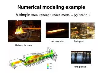
Numerical Modeling
Numerical Modeling. Benjamin Lamptey and Thomas Warner National Center for Atmospheric Research (Research Applications Laboratory) lamptey@ucar.edu April 2, 2007. Motivation. Offer great opportunity for improved forecasting Research tool:

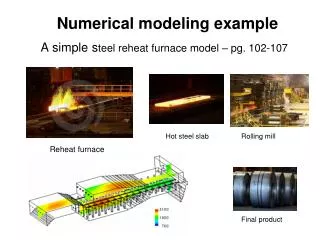
Numerical Modeling
E N D
Presentation Transcript
Numerical Modeling Benjamin Lamptey and Thomas Warner National Center for Atmospheric Research (Research Applications Laboratory) lamptey@ucar.edu April 2, 2007
Motivation • Offer great opportunity for improved forecasting • Research tool: • for weather research at all time-scales (including diurnal processes), • develop a model with parameterizations that properly reflect African conditions • Decision-making tool (what if scenarios) • A tool for cooperation among local universities, government agencies and the private sector regarding weather and climate information.
What is a Model? • Take the equations that describe atmospheric processes. • Convert them to a form where they can be programmed into a large computer. • Solve them so that this software representation of the atmosphere evolves within the computer. • This is called a “model” of the atmosphere
What do we mean by “solve the equations” • The equations describe how the atmosphere changes with time. • For example, one equation would be
So – “solving” the equation would be to estimate the terms on the right side, add them up, and obtain the rate of change of temperature
Similar Equations Would be Solved for • East-west wind component • North-south wind component • Specific humidity (or RH) • Pressure • Cloud water • Rain/snow water
Two Types of Models • Global – grid covers the entire atmosphere of Earth (global models) • Weather (GFS) • Climate (e.g. CCSM) • Limited-area – grid covers a region of the atmosphere such as continent or a state or a city (limited area models) • Weather (WRF, eta) • Climate (WRF,PRECIS,RegCM3)
Uses of Atmospheric Models • Daily weather prediction (let models run into the future for 1-10 days) • Climate prediction (let models run for years) - “what-if” experiments, e.g., what will happen if we double the CO2? - simply let the model run forward • Research – Study the model solution when you don’t have good observations of real atmosphere
Why WRF • It is free • It is a community-based model • Technical support by NCAR (wrfhelp@ucar.edu) • Rapid community growth • Two dynamical cores, numerous physics, chemistry • Has both operational and research capabilities
What can WRF be used for? • Operational NWP • Data Assimilation • Parameterized physics research • Downscaling climate simulations • Driving air-quality,agricultural, etc models
WRF Supported Platforms • MacOS • Linux • Unix (UNICOS, AIX, IRIX, Solaris)
Computing Resources • Single processor desktop • Dual core or quad desktop system • Linux cluster • Supercomputer -many processors
Why Important • Can be coupled to application models for • Agriculture • Water resources • Health • Energy • Transportation (aviation, turbulence, etc)
Research Questions What are the effects of these on the weather and climate? • Change in SSTs • Change in vegetation • Presence or absence of a lake • Irrigation system • Urbanization • Deforestation
What will you like to do with the model • Key points • Action items
CASE STUDY August 28, 2005 Mesoscale Convective System over West Africa
Some features of WRF-ARW • Nonhydrostatic with hydrostatic option • Two-way nesting with multiple nests and nest levels • One-way nesting • Vertical grid-spacing can vary with height • See Users Guide for more
Model • WRF version 2.1.2 • Grid resolution is 12 km, 4km • Grid size: 251x201, 216x196, 31 levels • BC and IC: NCEP and ECMWF • Period of simulation Aug. 27:00UTC to August 30:00UTC
Animation 1 BMJ WSM6 ECMWF
Animation 2 KF Lin et al. ECMWF
Animation 3 KF Thompson ECMWF
24-hour rain 6h-6h Aug 27 KF WSM6 ECMWF CPC WRF
24-hour rain 6h-6h Aug 28 KF WSM6 ECMWF WRF CPC
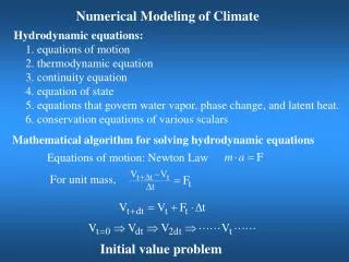
Governing Equations • Conservation of momentum or Newton’s 2nd law (3 equations for u,v,w) • Conservation of mass or continuity equation • First law of thermodynamics or conservation of energy • Equation of state for ideal gases • Moisture equation or a conservation equation for water mass
History of NWP • 1904 - Bjerknes (suggested use of hydrodynamic and thermodynamic equations), Richardson (hand-calculations) • After World War II - mathematical forecast possible (using Bjerknes suggestion). Simple forecasts in 1950s • 1962 - US launched first operational quasi-geostrophic baroclinic model, followed by Britain in 1965 • 1966 - First global PE model (NMC, Washington DC): 300km resolution, 6 vertical layers • http://www.ecmwf.int/products/forecasts/guide/The_history_of_NWP.html • Idealized simulations (PBL eddies, convection, baroclinic waves)
Model Web sites Real-Time Demonstration home page http://www.ral.ucar.edu/projects/wafrica 4DWX home page http://www.rap.ucar.edu/projects/4DWX References page http://www.rap.ucar.edu/projects/armyrange/references.html