Download
1 / 1
10 likes | 95 Vues
Explore Arctic hydrological processes using an ensemble of five land surface models to estimate key variables. A Bayesian Model Averaging approach is applied to enhance predictions.

E N D
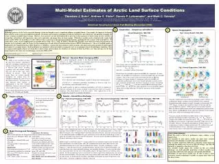
Multi-Model Estimates of Arctic Land Surface Conditions Theodore J. Bohn1, Andrew G. Slater2, Dennis P. Lettenmaier1, and Mark C. Serreze2 1Department of Civil and Environmental Engineering, Box 352700, University of Washington, Seattle, WA 98195 2Cooperative Institute for Research in Environmental Sciences, 216 UCB, University of Colorado, Boulder, CO 80309-0216 American Geophysical Union Fall Meeting (December 2005) 6 7 Evaporation – Comparison with ERA-40 Spatial Disaggregation ABSTRACT Hydrologic processes in the Arctic terrestrial drainage system are thought to exert a significant influence on global climate. For example, the impact of freshwater fluxes into the Arctic ocean on the global thermohaline circulation and the positive atmospheric feedback exhibited by snow albedo have the potential to amplify the Arctic's response to global climate change. However, these processes are not well understood, in part due to the sparseness of observations of such variables as stream flow, soil moisture, soil temperature, snow water equivalent, and energy fluxes in Arctic regions. While these variables can be estimated with a single land surface model (LSM), the predictions are often subject to biases and errors in the input meteorological forcings and limited by the accuracy of the model physics. To reduce these errors, we have implemented an ensemble of five LSMs: VIC1, CLM2, ECMWF3, NOAH4 and CHASM5, all of which have been used previously to simulate Arctic hydrology under the Project for Intercomparison of Land-surface Parameterization Schemes (PILPS) Experiment 2e.The use of multiple models is facilitated by the Standard Interface Multi- Model Array (SIMMA), a framework that automates model execution, data processing, and translation of model inputs and outputs to a common format. Model predictions are combined via Bayesian model averaging to arrive at an optimum estimate of hydrological conditions. Here we compare multi-model estimates of stream flow to observations and investigate the robustness of estimates of latent heat fluxes over time and space for the four largest basins in the Arctic terrestrial drainage system from 1980 to 1999. 1Variable Infiltration Capacity macroscale model (Liang et al., 1994) 4NCEP, OSU, Air Force, and NWS Hydrologic Research Lab collaborative model 2Community Land Model (NCAR & UCAR) 5CHAmeleon Surface Model 3European Center for Medium-range Weather Forecasting, land component of Integrated Forecast System model Annual Evaporation, 1980-1999 Fig 1: Annual Runoff, 1980-1999 Lena Yenisei Ob MacKenzie 1 4 Models Method – Bayesian Model Averaging (BMA) • For a given hydrological variable Y, the Bayesian Model Averaging method (Raftery et al., 2005) yields not only an optimal estimate Xens but also a probability distribution p(Y|Xens) about that estimate, as follows: • Xens(t) = Σ wkX’k(t) • p(Y(t)|Xens(t)) = Σ wk p(Y(t)|X’k(t)) • where • X’k = bias-corrected output of model k • wk = weight of model k • Y(t) = observed value of hydrological variable Y, during some training period • p(Y(t)|X’k(t)) = conditional probability distribution of observed value Y(t) given the bias-corrected model result X’k(t) • The model weights wk and the conditional probabilities p(Y(t)|X’k(t)) depend on both the correlation of the results of model k with observed values of Y and the frequency with which model k is the best model. Note: implicit here is the assumption that X and Y are normally-distributed. The LSMs in our ensemble all share the same basic structure, consisting of grid cells containing a multi-layer soil column overlain by one or more “tiles” of different land covers, including vegetation with and without canopy, bare soil, and in some cases, lakes, wetlands, or glaciers. Water and energy fluxes are tracked vertically throughout the column from the atmosphere through the land cover to the bottom soil layer. The figure to the right illustrates these features as implemented in the VIC (Variable Infiltration Capacity) macroscale land surface model (Liang et al., 1994). • Since storage terms are negligible in the annual water budget, we computed ensemble estimates of evaporation as: • Eens = P – Rens • where Rens = ensemble estimate of discharge. • Plotted above are ensemble evaporation and ERA-40 evaporation. It can be clearly seen that ERA-40 evaporation is consistently higher than our ensemble estimates. This is due, in part, to the consistently low bias of ERA-40 discharge (see figures in panel 5), and in part, to the fact that ERA-40 evaporation and discharge sum to more than precipitation (an artifact of the data assimilation method used). For better comparison, we have also plotted (P – Rera40_bc), where Rera40_bc is the bias-corrected ERA-40 discharge from panel 5, below. (P – Rera40_bc) comes much closer to our ensemble estimate, almost always falling within the 10th and 90th percentiles of the ensemble distribution. Fig 2: Annual Evaporation, 1980-1999 For the current demonstration we have selected three of the five models in the ensemble: VIC, NOAH, and CHASM. 2 5 Results – Annual River Discharge Region of Study We focused on the four largest river basins draining into the Arctic Ocean: Lena 2430000 km2 Yenisei 2440000 km2 Ob 2950000 km2 MacKenzie 1680000 km2 Fig 1: Raw Annual Discharge, 1980-1999 Fig 2: Bias-Corrected Discharge, 1980-1999 Fig 3: Ensemble Discharge, 1980-1999 Using the weights derived for total basin discharge (panel 5, below), we combined the models’ estimates of local runoff to form a spatially-distributed ensemble estimate of runoff, averaged over the period 1980-1999. Figure 1 compares the ensemble estimate to both raw and bias-corrected ERA-40 estimates. With respect to our ensemble estimates, ERA-40 tends to underestimate runoff in the mountainous portions of the Lena, Yenisei, and MacKenzie basins and in the lowlands near the mouth of the Lena; while overestimating runoff elsewhere. Using our spatially-distributed ensemble runoff, we then computed spatially-distributed ensemble evaporation as Eens = P – Rens. Figure 2 compares this to ERA-40 evaporation and P – (Rera40_bc). It can be seen that ERA-40 overestimates evaporation consistently, with respect to our ensemble. However, the general spatial patterns of both estimates of evaporation are similar, reaching maxima in the Ob, southern Lena, and southern MacKenzie basins, and minima in the northern Lena and Yenisei basins, where cold temperatures predominate. Lena Yenisei Lena Yenisei Lena Yenisei Ob MacKenzie Ob MacKenzie Ob MacKenzie Figure 1 shows simulated and observed annual discharge in the four major Arctic river basins. Annual discharge from the ERA-40 analysis is shown for comparison. The individual models, as well as the ERA-40 estimates, have substantial biases that differ from basin to basin. After bias correction (figure 2), the individual models (and ERA-40) agree much more closely with observed discharge. Figure 3 shows the ensemble mean and 10th and 90th percentiles. Note the narrow ensemble distribution for the Ob basin, indicating a robust estimate. Model weights are plotted in figure 4. Clearly, models do not contribute equally to the ensemble, and their contributions vary with location, with VIC performing best in the Lena and Ob basins, and CHASM performing best in the Yenisei and MacKenzie basins. NOAH’s contribution is small. Figures 5 -7 show the annual means, standard deviations, and rms errors of observed discharge, raw model discharge, bias-corrected model discharge, and ensemble discharge. It can be seen that while bias correction reduces the rms error of the model estimates, the improvement is not uniform across models. Yet the ensemble rms error is consistently less than or equal to the minimum rms error among the bias-corrected models. The rms error varies across basins and is much lower for the Ob than for the other basins. It should also be noted that, while ERA-40 discharge has large disagreement with observations, it becomes competitive when bias-corrected. 3 Fig 4: Model Weights Fig 5: Annual Means Model Forcings and Parameters • Forcing • ERA-40 Precipitation, Air Temperature, Surface Pressure, Humidity, Wind, and Radiation • Resampled to 100km EASE (equal area) grid • Disaggregated to 3-hour intervals, 1979-1999 • Initialization • Soil temperature initialized to 273 K • Soil moisture initialized to saturation • First year (1979) treated as spin-up • Internal time step • VIC: 3 hours; others: 30 minutes • Land Surface Parameters • Different models have different requirements • Soil: FAO or Zobler soil types • Land cover: from University of Maryland 1-km Global Land Cover • Some models handle glaciers, lakes, and wetlands while others do not • Number of land cover tiles per grid cell varies from 1 (NOAH) to 4 or more (VIC and CLM) • Number of soil and snow layers varies from model to model • Note: Models were not calibrated for these forcings. • CONCLUDING REMARKS • While this study is still in its preliminary stages, evidence so far suggests that: • An ensemble of land surface models can make more accurate predictions of hydrological variables than individual models. • Our ensemble outperforms ERA-40 in estimating annual discharge (although the models were driven by ERA-40 forcings, and ERA-40 discharge is competitive when bias-corrected). • An ensemble trained against one variable (in this case annual discharge) can make plausible predictions of other variables (e.g. evaporation, both basin-wide aggregate and spatially-distributed). • Ensembles of land surface models may be able to help us more accurately estimate hydrological variables in regions where there are few observations. • Note: See the author for a list of references. Fig 6: Standard Deviations Fig 7: RMS Error