Parameterization of land surface
Parameterization of land surface . Bart van den Hurk (KNMI/IMAU). Last week: Orders of magnitude. Estimate the energy balance of a given surface type What surface? What annual cycle? How much net radiation? What is the Bowen ratio (H/LE)? How much soil heat storage?

Parameterization of land surface
E N D
Presentation Transcript
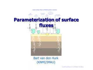
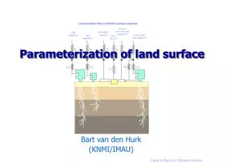
Parameterization of land surface Bart van den Hurk (KNMI/IMAU) Land surface in climate models
Last week: Orders of magnitude • Estimate the energy balance of a given surface type • What surface? • What annual cycle? • How much net radiation? • What is the Bowen ratio (H/LE)? • How much soil heat storage? • Is this the complete energy balance? • The same for the water balance • How much precipitation? • How much evaporation? • How much runoff? • How deep is the annual cycle of soil storage? • And the snow reservoir? Land surface in climate models
General setup of General Circulation Models (3) • Many processes are sub-grid, and need to be parameterized • Fine scale processes (fluxes) expressed in terms of resolved variables (mean state) using (semi-) empirical, observation based equations • Example: turbulent sensible heat flux a a H H = Sensible heat flux [W/m2] = air density [kg/m3] cp = specific heat [J/kg K] U = wind speed [m/s] CH = exchange coefficient [-] s - a = temperature gradient [K] s s Land surface in climate models
General form of land surface schemes P E Q* H LE Rs Infiltration D G • Energy balance equation K(1 – a) + L – L + E + H = G • Water balance equation W/t = P – E – Rs – D Land surface in climate models
General form of land surface schemes P E Q* H LE Rs Infiltration D G • Energy balance equation K(1 – a) + L – L + E + H = G • Water balance equation W/t = P – E – Rs – D • Coupled via the evaporation Land surface in climate models
Land surface heterogeneity • Land surface is heterogeneous blend of vegetation at many scales • forest/cropland/urban area • within forest: different trees/moss/understories • Most LSMs use set of parallel “plant functional types” (PFTs) with specific properties • gridbox mean or tiled • Some ecological models treat species competition and dynamics within PFTs • Properties of PFTs • LAI • rooting depth • roughness • albedo • emission/absorption of organic compounds Land surface in climate models
Development history of land schemes • Late 1960’s: bucket scheme (Manabe, 1969) with depth of the reservoir = 15cm P E Direct runoff E = (W/Wmax) Epot R = 0 (W<Wmax) R = P – LE (WWmax) Land surface in climate models
Penman Monteith equation • Given: • The Penman-Monteith equation can be derived: Land surface in climate models
Development history of land schemes • Mid 1970’s: explicit treatment of vegetation (Penman-Monteith ‘big leaf’) • To be combined with submodel for soil infiltration/runoff P E Direct runoff Land surface in climate models
First Soil-Vegetation-Atmosphere Scheme (SVAT) • Deardorff (1978) combined • Penman-Monteith • Partial vegetation coverage, but still one energy balance equation (lumped surface types) • ‘effective’ surface resistance (interpolating between canopy value for full vegetation, and large value for bare ground) Land surface in climate models
Explicit multi-component SVATs • Separate treatment of vegetation and understory/bare ground (Shuttleworth et al, 1988) • canopy resistance • evap. resistance for bare ground • Complex rewriting of PM, involving • separate net radiation for two components • solution of T,q “within canopy” (at network node) • separate aerodynamic coupling of two components • Evaporation at bare ground affects canopy transpiration and vice versa Land surface in climate models
Tiled scheme • For instance ECMWF (2000) • Multiple fractions (“tiles”) • vegetation (transpiration) • bare ground (evaporation) • interception/skin reservoir (pot. evaporation) • snow (sublimation) • Multi-layer soil • diffusion • gravity flow • Explicit root profile Land surface in climate models
Structure of a land-surface scheme (LSS or SVAT) • 6 fractions (“tiles”) • Aerodynamic coupling • Vegetatie • Verdampingsweerstand • Wortelzone • Neerslaginterceptie • Kale grond • Sneeuw Land surface in climate models
Structure of a land-surface scheme (LSS or SVAT) • 6 fractions (“tiles”) • Aerodynamic coupling • Wind speed • Roughness • Atmospheric stability • Vegetatie • Verdampingsweerstand • Wortelzone • Neerslaginterceptie • Kale grond • Sneeuw Land surface in climate models
Structure of a land-surface scheme (LSS or SVAT) • 6 fractions (“tiles”) • Aerodynamic coupling • Wind speed • Roughness • Atmospheric stability • Vegetation • Canopy resistance • Root zone • Interception • Kale grond • Sneeuw Land surface in climate models
Structure of a land-surface scheme (LSS or SVAT) • 6 fractions (“tiles”) • Aerodynamic coupling • Wind speed • Roughness • Atmospheric stability • Vegetation • Canopy resistance • Root zone • Interception • Bare ground • Sneeuw Land surface in climate models
Structure of a land-surface scheme (LSS or SVAT) • 6 fractions (“tiles”) • Aerodynamic coupling • Wind speed • Roughness • Atmospheric stability • Vegetation • Canopy resistance • Root zone • Interception • Bare ground • Snow Land surface in climate models
Components discussed • Definition of vegetation • Canopy resistance • Aeordynamic exchange and numerical solution • Soil water and runoff • Snow Land surface in climate models
Maps of PFTs • Based on remote sensing/local inventories • Available at high resolution (1km) • Various versions produced for different PFT-classifications • Global Land Cover Climatology (GLCC) • ECOCLIMAP Area (VIS) (NIR) NDVIJJA NDVIDJF Pine forest low high high high Deciduous forest low high high low Grassland middle high middle middle Crops middle high high low Bare soil high low low low Land surface in climate models
Vegetation distribution Land surface in climate models
Global distribution of forest/low vegetation in HTESSEL Land surface in climate models
Specification of vegetation types Land surface in climate models
The coupled CO2 – H2O pathway in vegetation models • qin = qsat(Ts) • Traditional (“empirical”) approach: rc = rc,min f(LAI) f(light) f(temp) f(RH) f(soil m) Land surface in climate models
More on the canopy resistance • Active regulation of evaporation via stomatal aperture • Two different approaches • Empirical (Jarvis-Stewart) rc = (rc,min/LAI) f(K) f(D) f(W) f(T) • (Semi)physiological, by modelling photosynthesis An = f(W) CO2 / rc An = f(K, CO2) CO2 = f(D) Land surface in climate models
Jarvis-Stewart functions • Shortwave radiation: • Atmospheric humidity deficit (D): f3 = exp(-cD) (c depends on veg.type) Land surface in climate models
Jarvis-Stewart functions • Soil moisture (W = weighted mean over root profile): • Standard approach: linear profile f2 = 0 (W < Wpwp) = (W-Wpwp)/(Wcap-Wpwp) (Wpwp<W<Wcap) = 1 (W > Wcap) • Alternative functions (e.g. RACMO2) Lenderink et al, 2003 Land surface in climate models
Carbon exchange • Carbon & water exchange is coupled • Carbon pathway: • assimilation via photosynthesis • storage in biomass • above ground leaves • below ground roots • structural biomass (stems) • decay (leave fall, harvest, food) • respiration for maintenance, energy etc • autotrophic (by plants) • heterotrophic (decay by other organisms) Land surface in climate models
Modelling rc via photosynthesis • An = f(soil m) CO2 / rc • Thus: rc back-calculated from • Empirical soil moisture dependence • CO2-gradient CO2 • f(qsat – q) • Net photosynthetic rate An • An,max • Photosynthetic active Radiation (PAR) • temperature • [CO2] Land surface in climate models
Aerodynamic exchange • Turbulent fluxes are parameterized as (for each tile): • Solution of CH requires iteration: • CH = f(L) • L = f(H) • H = f(CH) a Ta+gz a H s s L = Monin-Obukhov length Land surface in climate models
Numerical solution • Solution of energy balance equation • With (all fluxes positive downward) • Express all components in terms of Tsk (with Tp = Tskt -1) netradiation sensible heat flux latent heat flux soil heat flux Land surface in climate models
Effective rooting depth • Amount of soil water that can actively be reached by vegetation • Depends on • root depth (bucket depth) • stress function • typical time series of precip & evaporation • See EXCEL sheet for demo Land surface in climate models
Soil heat flux • Multi-layer scheme • Solution of diffusion equation • with • C [J/m3K] = volumetric heat capacity • T [W/mK] = thermal diffusivity • with boundary conditions • G [W/m2] at top • zero flux at bottom Land surface in climate models
Heat capacity and thermal diffusivity • Heat capacity • sCs 2 MJ/m3K, wCw 4.2 MJ/m3K • Thermal diffusivity depends on soil moisture • dry: ~0.2 W/mK; wet: ~1.5 W/mK Land surface in climate models
Soil water flow • Water flows when work is acting on it • gravity: W = mgz • acceleration: W = 0.5 mv2 • pressure gradient: W = m dp/ = mp/ • Fluid potential (mechanical energy / unit mass) • = gz + 0.5 v2 + p/ p = gz • g(z+z) = gh • h = /g = hydraulic head = energy / unit weight = • elevation head (z) + • velocity head (0.5 v2/g) + • pressure head ( = z = p/g) Land surface in climate models
Relation between pressure head and volumetric soil moisture content strong adhesy/ capillary forces water held by capillary forces retention curve Land surface in climate models
Parameterization of K and D • 2 ‘schools’ • Clapp & Hornberger ea • single parameter (b) • Van Genuchten ea • more parameters describing curvature better • Defined ‘critical’ soil moisture content • wilting point ( @ = -150m or -15 bar) • field capacity ( @ = -1m or -0.1 bar) • Effect on water balance: see spreadsheet Land surface in climate models
pF curves and plant stress • Canopy resistance depends on relative soil moisture content, scaled between wilting point and field capacity clay organic sand Land surface in climate models
Boundary conditions • Top: F [kg/m2s] = T – Esoil – Rs + M • Bottom (free drainage) F = Rd = wK • with • T = throughfall (Pl – Eint – Wl/t) • Esoil = bare ground evaporation • Eint = evaporation from interception reservoir • Rs = surface runoff • Rd = deep runoff (drainage) • M = snow melt • Pl = liquid precipitation • Wl = interception reservoir depth • S = root extraction Pl Eint T Wl Esoil M Rs S Rd Land surface in climate models
Parameterization of runoff • Simple approach • Infiltration excess runoff Rs = max(0, T – Imax), Imax = K() • Difficult to generate surface runoff with large grid boxes • Explicit treatment of surface runoff • ‘Arno’ scheme Infiltration curve (dep on W and orograpy) Surface runoff Land surface in climate models
Snow parameterization • Effects of snow • energy reflector • water reservoir acting as buffer • thermal insolator • Parameterization of albedo • open vegetation/bare ground • fresh snow: albedo reset to amax (0.85) • non-melting conditions: linear decrease (0.008 day-1) • melting conditions: exponential decay • (amin = 0.5, f = 0.24) • For tall vegetation: snow is under canopy • gridbox mean albedo = fixed at 0.2 Land surface in climate models
Parameterization of snow water • Simple approach • single reservoir • with • F = snow fall • E, M = evap, melt • csn = grid box fraction with snow • Snow depth • with • sn evolving snow density (between 100 and 350 kg/m3) • More complex approaches exist (multi-layer, melting/freezing within layers, percolation of water, …) Land surface in climate models
Snow energy budget • with • (C)sn = heat capacity of snow • (C)i = heat capacity of ice • GsnB = basal heat flux (T/r) • Qsn = phase change due to melting (dependent on Tsn) Land surface in climate models
Snow melt • Is energy used to warm the snow or to melt it? In some stage (Tsn 0C) it’s both! • Split time step into warming part and melting part • first bring Tsn to 0C, and compute how much energy is needed • if more energy available: melting occurs • if more energy is available than there is snow to melt: rest of energy goes into soil. Land surface in climate models
Next week • How would a parameterization scheme for irrigation look like? • External (static) variables • Resolved variables (boundary conditions) • Prognostic quantities • Main processes Land surface in climate models
More information • Bart van den Hurk • hurkvd@knmi.nl Land surface in climate models