Understanding Fourier Transformations: Forward, Inverse, and Applications
This text delves into the principles of Fourier transformations, including forward and inverse transformations, and their applications in various fields such as signal processing and optics. We explore the relationship between time and frequency domains, explaining complex functions, Fourier spectra, and phase angles. The document also covers convolution, point spread functions in imaging, and the discrete Fourier transformation (DFT), highlighting the efficiency of the Fast Fourier Transformation (FFT). Lastly, we touch upon continuous wavelet transforms and their significance in analyzing complex signals.

Understanding Fourier Transformations: Forward, Inverse, and Applications
E N D
Presentation Transcript
Transformations Theo Schouten
Fourier transformation forward inverse f(t) = cos(2**5*t) + cos(2* *10*t) + cos(2* *20*t) + cos(2* *50*t) Theo Schouten
Spectrum, phase In general F(u) is a complex function: F(u) = R(u) + j I(u) = | F(u) | ej (u) | F(u) | = (R2(u) + I2(u) ) : the Fourier spectrum of f(x)(u) = tan-1 ( I(u) / R(u) ) : the phase angle of f(x) Theo Schouten
2 D Fourrier F(u,v) = f(x,y) e-j2(ux+vy) dx dyf(x,y) = F(u,v) e+j2(ux+vy)du dv Theo Schouten
Convolution • c(x) = f(x) g(x) = f()g(x-) d • C(u) = F(u)G(u) • Point spread function of a lens • Light on ideal point (,) spread over pixels (x,y) according h(x,,y, ) • p(x,y) = w (,) h(x,,y, ) d d • Linear: h(x,,y, ) = h(x-,y- ) • p(x,y) = w (,) h(x-,y- ) d d = w h • P(u,v) = W(u,v)H(u,v) Theo Schouten
Discrete Fourier Transformation In 2-D the DFT becomes: F[u,v] = 1/MN x=0M-1y=0 N-1 f[x,y]e -j2 (xu / M + yv / N)f[x,y] = u=0M-1v=0N-1 F[u,v] e+j2(xu / M + yv / N) Theo Schouten
Fast Fourier Transformation • To calculate F[u] for u=0,1...N-1 it takes N*N multiplications and N*(N-1) summations of complex numbers (e... in a table). • The complexity of a DFT is therefore proportional to N2. • Transform 1 DFT of N terms into 2 DFTs of N/2 terms. • We can apply this recursively and reach a complexity of N log2N. • special purpose hardware chips wirh parallel processing Theo Schouten
Use in CT g (x') = f(x',y') dy' x' = x cos + y sin y'= -x sin +y cos FT( g (x')) = F(u cos , u sin ). Theo Schouten
Other transformations • DFT example of whole class of transformations • T(u) = x=0 N-1 f(x) g(x,u) with g the forward transformation kernelf(x) = u=0 N-1 T(u) h(x,u) with h the inverse transformation kernel • Discrete Cosine: cos( (2x+1)u / 2N) , JPEG, MPEG • T(u,v) = x=0 N-1y=0 N-1 f(x,y) g(x,y,u,v)f(x,y) = u=0 N-1v=0 N-1 T(u,v) h(x,y,u,v) • g(x,y,u,v) = g1(x,u) g2(y,v) : separable: 2D = N 1D Theo Schouten
Continuous wavelets Mexican-hat (x)= c (1-x2) exp(-x2/2) the second derivative of a Gaussian Construction of the Morlet wavelet as a sinus modeled by a Gaussian function • set of wavelet basis functions s,t(x) : • s,t(x) = ( (x-t) / s) / s, s > 0 the scale and t the translation • The CWT of f(x) is then: • Wf(s,t) = <f, s,t> = f(x) s,t(x) dx • f(x) = (1 / C ) Wf(s,t) s,t(x) dt ds/s2 Theo Schouten
Continuous wavelet transform Theo Schouten
Time frequency tilings In the discrete wavelet transform one works with factors 2 Also here there is a Fast Wavelet Transformation Theo Schouten
Example 3 scale 2D FWT Theo Schouten
Example Theo Schouten