Download
1 / 42
430 likes | 613 Vues
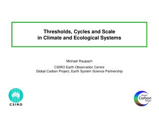
Thresholds, Cycles and Scale in Climate and Ecological Systems. Michael Raupach CSIRO Earth Observation Centre Global Carbon Project, Earth System Science Partnership. Outline. Plan Introduction – some thoughts on thresholds and scale Climate: ice age thresholds

E N D
Thresholds, Cycles and Scalein Climate and Ecological Systems Michael Raupach CSIRO Earth Observation CentreGlobal Carbon Project, Earth System Science Partnership
Outline • Plan • Introduction – some thoughts on thresholds and scale • Climate: ice age thresholds • A system where large-scale thresholds are driven by self-organisation and modulated by external forcing • Ecological optimality: steady state and dynamic perspectives • Short term (dynamic, small scale) threshold behaviour can disappear in long time scales (steady state, large scale)
Thresholds at small and large scales • Most of the systems we study have small-scale and large-scale dynamics • Often (not always) we try to infer large-scale dynamics (emergent properties) from small-scale dynamics • Small-scale dynamics Large-scale dynamics • Relationship between phenomenological laws [f(x)] at small and large scales: f F f F x x prob(x) prob(x) x x
Thresholds at small and large scales • Linear systems: F(X) (large) is identical with f(x) (small) Nonlinear systems: F(X) (large) is a blurred version of f(x) (small) • Thresholds in f(x) (small) do not translate into thresholds in F(X) or X(t) (large) • Most large-scale threshold phenomena are emergent dynamical properties of the large-scale system itself – cannot be inferred directly from small-scale laws • Can study large-scale emergent system behaviour (including possible thresholds) EITHER by integrating dx/dt = f(x), then finding X(t) = <x(t)> OR by inferring F(X), then integrating dX/dt = F(X)
Climate thresholds Ice-age temperature records: • Vostok oscillations: Period around 100 ky • Dansgaard-Oescher (DO) oscillations: variable period, typically a few ky
Simplified climate model for DO oscillations(Rial 2005, following Saltzman, 1983 to 2004) • Ice-core temperatures in Greenland
Frequency-modulated astable oscillator • Mechanism for generating a sawtooth waveform • No external trigger required for threshold events • Externally driven variation in threshold level (Milenkovich) changes the frequency of threshold events
The Milenkovich cycles Tilt or obliquity41,000 years Eccentricity41,000 years Precession of the equinoxes23,000 years
Simplified climate model for DO oscillations(Rial 2005, following Saltzman, 1983 to 2004) • Saltzman nonlinear thermal oscillator with Milenkovich forcing • Energy balance equation for mean atmospheric temperature (T) • Logistic equation for sea ice extent (L) • These together yield a van der Pol equation for L (with Milenkovich forcing) • van der Pol equation gives self-excited oscillations with a limit cycle • Milenkovich forcing modulates the frequency of these oscillations
Simplified climate model for DO oscillations(Rial 2005, following Saltzman, 1983 to 2004)
Simplified climate model for DO oscillations(Rial 2005, following Saltzman, 1983 to 2004)
Climate thresholds: summary • The planetary climate of Earth is dynamic: abrupt changes are the norm • Changes typically have a threshold-like character (fast warming, slow cooling) • Thresholds are driven by self-organisation (limit cycle in a nonlinear system), and are modulated by external forcing • Self-organisation (endogenous drivers) • Ice, oceans, CO2, dust, plants • Vulcanism-carbonate cycle • Continental drift • External forcing (exogenous drivers) • Orbital forcing • Meteorites
Ecological optimality • Ecological Optimality Hypothesis (EOH): • evolutionary selection pressures drive ecosystems towards a state of maximum utilisation of available resources (light, water, nutrient) for biomass production, • so that long-term net primary production (NPP) over many reproductive cycles takes the largest possible value under the constraints of available resources. • Three versions: • Plant functional optimality (Cowan 1977, Cowan and Farquhar 1977) • Hydroecological optimality (Eagleson 1978, 2002) • Resource use optimality and the resource balance hypothesis (Mooney and Gulmon 1979,. Field 1991, Field et al 1995)
Unconstrained and constrained optimisation • Steady (find an optimum point) • (U) Find the top of the hill • (C) Get as close as possible to the top of the hill when you can only move along a prescribed line • Dynamic (find the best path in time) • (U) Find a path from A to B which maximises your average height • (C) Find a path from A to B which maximises your average height when you also have to satisfy dynamic constraints • In optimisation problems, constraints are not add-ons or afterthoughts; they are fundamental aspects of the problem
Optimality in the steady state • Problem: • Solution: use a Lagrange multiplier to define a Lagrangian (L) and thus turn the constrained maximisation problem into an unconstrained problem:
Optimality in the steady stateResource Balance Hypothesis (Field et al 1993; Schimel, Parton et al 1995) • Example: find C stores [(C1, C2) = (leaf C, root C)] which maximise production [G] • The steady-state mass balance is: dC/dt = G(C) – k.C = 0 • We are given the production G(C), and a vector k of decay rates for C1, C2 Contours of G(C) Resource-balance curve: curve along which grad G(C) is parallel to k[or k is normal to contour of G(C)] Optimising solution: • constraint curve is tangent to G(C)contours • all acquired resources are equally limiting (Resource Balance Hypothesis) C2(root C) Constraint curve [G(C) – k.C = 0]: • set of possible steady states • allocation ratio varies along this curve C1 (leaf C)
Application 1Dependence of leaf/root allocation on soil moisture • Two carbon stores: (leaf C, root C) = (CL, CR) • Growth C flux G(CL, CR) (= Net Primary Production) is the parallel sum of fluxes limited by light (Q) and water (W). This implies • Analytic result for steady-state allocations to leaf (AL) and root (AR = 1 – AL): Potential water flux (ET) Incident light flux Response of GQLim to CL Light use efficiency Response of GWLim to CR Water use efficiency
Application 1Dependence of leaf/root allocation on soil moisture • Analytic result for steady-state allocations to leaf (AL) and root (AR = 1 – AL):
Application 2Effect of agriculture on Australian Net Primary Production • Australian NPP without agricultural inputs of nutrients and water • Ratio: (NPP with agric) / (NPP without agric) • Largest local NPP changes: around x 2 • Continental change in C cycle: 1.07 • Continental change in N cycle: around 2 Raupach, M.R., Kirby, J.M., Barrett, D.J., Briggs, P.R., Lu, H. and Zhang, L. (2002). Balances of water, carbon, nitrogen and phosphorus in Australian landscapes: Bios Release 2.04. CD-ROM (19 April 2002). CSIRO Land and Water.
Dynamic optimisation: the Minimum Principle • A general dynamic constrained optimisation problem:
Dynamic optimisation: the Minimum Principle • Solution: The Pontryagin Minimum Principle • So we have to find the costate variables (t), then the Hamiltonian h(x,u,), then choose the control variables u(t) which minimise h at each point in time • When the system is linear in the controls, the optimal controls are "bang-bang":the optimal u(t) switches between limiting component values umin and umax
Applications of the Minimum Principle • Basic Calculus of Variations: • Lagrange and Hamilton formulations of classical mechanics: • Data assimilation, model-data fusion: Estimation of initial conditions (x0)Estimation of parameters (u)
Example: allocation to biomass and seed • Mass balance equations: • C pools: (biomass, seed) = (c1, c2) • Objective: maximise seed biomass (c2) after 1 cycle (year) with b = (0,1) = weight vector for C pools in goal function • Hamiltonian: • Control variable: allocation to biomass = a1 (with a2 = 1 – a1) • Switching criterion: • maximise h with respect to a • Implying a1 = 1 when 1 – 2 – 1 > 0, and a1 = 0 otherwise
a1 c2 1 c1 h time 2 Switch = 1 – 2 – 1 Example: allocation to biomass and seed • Costate variables (1, 2) are marginal benefits of investment in (c1, c2) • Hamiltonian h is constant in time for the optimum solution
Summary • Scale • Small-scale and large-scale threshold phenomena are subtly connected • Small scale thresholds appear directly at large scales only in blurred form • Most large-scale threshold phenomena are emergent dynamical properties of the large-scale system itself – cannot be inferred directly from small-scale laws • Climate oscillations • Ice-age dynamics (DO oscillations) – thresholds result from self-organisation (a limit cycle in a nonlinear system), and are modulated by external forcing • Ecological optimality • Contrasting steady state and dynamic perspectives • Short term (dynamic, small scale) threshold behaviour can disappear in long time scales (steady state, large scale) • Implications for the coupled climate-carbon-human system • We don't know what is in store, so it is very important(1) to keep watching the horizons (better observations)(2) to improve our future navigation (better models)
Climate thresholds Ice-age temperature records: • Vostok oscillations • Period around 100 ky • Dansgaard-Oescher (DO) oscillations • Variable period, typically a few ky
Global warming • IPCC (2001) • Predicted warming of 1.4 to 5.8 C depends on (1) uncertainties in climate models (around 1 C) (2) uncertainties in emissions scenarios (around 2 C) IPCC (2001) Third Assessment, Summary for PolicyMakers
SCOPE-GCP Rapid Assessment of the Carbon Cycle • Field CB, Raupach MR (eds.) (2004) The Global Carbon Cycle: Integrating Humans, Climate and the Natural World. Island Press, Washington D.C. 526 pp. • GlobalCarbonProject.org
Fire and respiration feedbacks Absent Present Global Land C 8 Atmospheric CO2 Global Temperature 1000 6 2°C 200 ppm 800 4 600 2 400 0 -2 200 1850 1900 1950 2000 2050 2100 1900 1950 2000 2050 2100 Vulnerable carbon pools in the 21st centuryC emissions from land biomes • x Cox et al. (2000)
Simplified terrestrial biogeochemical modela two-component dynamical system with fast and slow stores • Stores: (x1, x2) = (FastStore, SlowStore), say (LeafCarbon, SoilNutrient) • Random forcing: F(t) is log-Markovian, mean = 1, SDev/mean = 0.5Parameters: p1 = 1, p2 = 1 = scales for effect of x1 and x2 limitation on production k1 = 0.2, k2 = 0.1 = rate constants for fast, slow pools (inverse time units) s0 = 0.01 = seed production (constant) • Optimisation Intercomparison (OptIC): comparative evaluation of parameter estimation and data assimilation methods for determining parameters in BGC models • GlobalCarbonProject.org
Threshold behaviourExternally forced system flips between "active" and quiescent" stable states Fwd01: k1=0.2 (default) Fwd03: k1=0.4 Fwd04: k1=0.5
Optimality in the steady stateResource Balance Hypothesis (Field et al 1993; Schimel, Parton et al 1995) • Example: find C stores [(C1, C2) = (leaf C, root C)] which maximise production [G] • The steady-state mass balance is: dC/dt = G(C) – k.C = 0 • Production is a minimum function: G(C) = min[G1(C1), G2(C2)] Contours of G(C) Resource-balance curve: G1(C1) = G2(C2) We don't have to find grad G(C)! Optimising solution: • constraint curve is tangent to G(C)contours • all acquired resources are equally limiting (Resource Balance Hypothesis) C2(root C) Constraint curve [G(C) – k.C = 0]: • set of possible steady states • allocation ratio varies along this curve C1 (leaf C)
Application 1Dependence of leaf/root allocation on soil moisture • State space diagram Resource-balance curve Constraint curve
Details • Raupach, M.R. (2005). Dynamics and optimality in coupled terrestrial energy, water, carbon and nutrient cycles. In: Prediction in Ungauged Basins (PUB): Australia-Japan perspectives (Eds. S. Franks, M. Sivapalan, Takeuchi, Tachikawa). (IAHS Press, Wallingford, UK). (In press). • Figure 1: Geometrical interpretation of the optimal (maximum-growth) solution for carbon pools (C1,C2) = (CL,CR) = (leaf, root). The dashed lines are the contours of the NPP G(C) on the (C1,C2) plane. The solid heavy line is the set of points (C1,C2) on which the carbon mass balance constraint, Equation (7), is satisfied. The dashed heavy line is the set of points (C1,C2) on which the gradient ∂G/∂Ci is parallel to the vector of decay rates, Ki. The optimum solution is at the intersection of the solid and dashed heavy lines, and is also the point at which the tangent to the constraint line (shown as a light solid line) is parallel to the contours of G(C). The contours for G(C) are constructed using Equation (12), with relative soil moisture W = 0.5 and other parameters as specified in the caption for Figure 2. With these parameters, G = 0.26 mol C m−2 d−1 at the optimum point. Contours are at intervals of 0.025 mol C m−2 d−1. • Figure 2: Allocation ratios predicted by Equation (14) as a function of equilibrium relative soil moisture W. Parameters in Equation (14) and the model for NPP G(C), Equation (12), are: light use efficiency αQ = 0.04 mol C mol PAR−1; water use efficiency αW = 0.005 mol C mol water−1; incident PAR flux FQx = 40 mol PAR m−2 d−1; proportionality constant relating soil-limited transpiration to relative water content FWx = 925 mol water m−2 d−1; scales for limitation of NPP and transpiration by lack of leaf and root, CL0 = 40 mol C m−2 and CR0 = 40 mol C m−2; leaf and root pool decay rates KL = 1 y−1 and KR = 0.5 y−1. • See also: Raupach, M.R., Barrett, D.J., Briggs, P.R. and Kirby, J.M. (2005). Terrestrial biosphere models and forest-atmosphere interactions. In: Prediction in Ungauged Basins (PUB): Australia-Japan perspectives (Eds. S. Franks, M. Sivapalan, Takeuchi, Tachikawa). (IAHS Press, Wallingford, UK). (In press).
Australian nitrogen balance and the effect of agriculture With agriculture Without agriculture N flux (kgN/m2/yr) Fert Dep FixGas Leach Disturb Raupach, M.R., Kirby, J.M., Barrett, D.J., Briggs, P.R., Lu, H. and Zhang, L. (2002). Balances of water, carbon, nitrogen and phosphorus in Australian landscapes: Bios Release 2.04. CD-ROM (19 April 2002). CSIRO Land and Water.
Primary production of biomass Respiration of biomass Extraction of biomass by humans Population growth rate Surplus in biomass extraction Human-biosphere interaction as a dynamical system A two-equation essentialist model • State variables: B(t) = biomass H(t) = human population • Equations: • Model for extraction of biomass by humans: • more humans extract more biospheric resource • each human extracts more as B increases (B is surrogate for quality of life) • A Lotka-Volterra system: familiar from dynamical ecology
Dynamical Systems 101 • Dynamical system: • Fixed points satisfy: • Determine stability of the solution near fixed points by solving the linearised system: • Solutions:
Application to the BH model • Linearised system: • Equilibrium point 1 (attractor when H=0): • characteristic equation • with solutions • Equilibrium point 2 (attractor when H=0): • characteristic equation • with solutions
Human-biosphere interaction as a dynamical system Trajectories on a (B,H) plane for 6 scenarios
Human-biosphere interaction as a dynamical systemTrajectories on a (B,H) plane with random climate variability in production Random primary production: log-Markovian, sd = 0.5, varying time scale
aB > (k/m)aH + kaE Q aB < (k/m)aH + kaE 1/c P/km A look at controllability • Question: can this system be managed for optimum quality of life? • Triple-bottom-line goal function (economy, environment, society): Quality (Q) = f(B,H) = aBB + aHH + aEE • Coefficients aB, aH, aE reflect the relative values placed on B (environment), H (society) and E (economy) in their contributions to Q • Adjust c to maximise Q at steady state (B=B2, H=H2) • Result: When aB > (k/m)aH + kaE: Q is maximum when H goes to 0 ("Eden") When aB < (k/m)aH + kaE: Q is maximum when B goes to 0 ("Exploit") • Unstable control ("bang-bang") control leads to threshold behaviour