
Hypothesis Testing
Hypothesis Testing. Make a tentative assumption about a parameter Evaluate how likely we think this assumption is true Null Hypothesis Default possibility H 0 : = 13 H 0 : = 0 Alternative (or Research) Hypothesis Values of a parameter if your theory is correct H A : > 13

Hypothesis Testing
E N D
Presentation Transcript
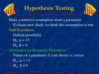
Hypothesis Testing • Make a tentative assumption about a parameter • Evaluate how likely we think this assumption is true • Null Hypothesis • Default possibility • H0: = 13 • H0: = 0 • Alternative (or Research) Hypothesis • Values of a parameter if your theory is correct • HA: > 13 • HA: 0
Hypothesis Testing • Test Statistic • Measure used to assess the validity of the null hypothesis • Rejection Region • A range of values such that if our test statistic falls into this range, we reject the null hypothesis • H0: = 13 • If x is close to 13, can’t reject H0. But if x is far away, then reject. But what’s “far away” ?? _ _
Hypothesis Testing Errors Action
Hypothesis Testing Errors Drug Testing Example H0: Not using drugs Action
Testing • A human resources executive for a huge company wants to set-up a self-insured workers’ compensation plan based on a company-wide average of 2,000 person-days lost per plant. A survey of 51 plants in the company reveals that x = 1,800 and s = 500. Is there sufficient evidence to conclude that company-wide days lost differs from 2,000? (Use = 0.05) _
If H0 is true… _ x has a t distribution with 50 degrees of freedom x = 2,000 _
When to Reject H0? _ x has a t distribution with 50 degrees of freedom Rejection Region P(rejection region) = _ _ x = 2,000 _ xL xUP
Testing • Suppose you are a human resources manager and are investigating health insurance costs for your employees. You know that five years ago, the average weekly premium was $30.00. You take a random sample of 40 of your employees and calculate that x = $31.25 and s = 5. • Have health care costs increased (use a 5% significance level)? _
If H0 is true… _ x has a t distribution with 39 degrees of freedom x = 30 _
When to Reject H0? _ x has a t distribution with 39 degrees of freedom P(rejection region) = Rejection Region _ x = 30 _ xUP
Important Note • Siegel emphasizes confidence intervals to do hypothesis tests • I do NOT want you to do it this way • It does not fit the logic that I will emphasize • It doesn’t fit with p-values • It’s too easy to get confused between one-tailed and two-tailed tests • So don’t follow Siegel, follow Budd
Testing p • An HR manager of a large corporation surveys 1,000 workers and asks “Are you satisfied with your job?” The results are ResponsesPercentage Satisfied 77% Not Satisfied 23% • You want to examine whether dissatisfaction is increasing. You know that the fraction of workers who were dissatisfied with their job five years ago was 20%. Has the fraction increased (at the 5% significance level)?
Regression • Recall Coal Mining Safety Problem • Dependent Variable: annual fatal injuries injury = -168.51 + 1.224 hours + 0.048 tons (258.82) (0.186) (0.403) + 19.618 unemp + 159.851 WWII (5.660) (78.218) -9.839 Act1952 -203.010 Act1969 (100.045) (111.535) (R2 = 0.9553, n=47) Test the hypothesis that the unemployment rate is not related to the injury rate (use =0.01)
Minitab Output Predictor Coef StDev T P Constant -168.5 258.8 -0.65 0.519 hours 1.2235 0.186 6.56 0.000 tons 0.0478 0.403 0.12 0.906 unemp 19.618 5.660 3.47 0.001 WWII 159.85 78.22 2.04 0.048 1952Act -9.8 100.0 -0.10 0.922 1969Act -203.0 111.5 -1.82 0.076 S = 108.1 R-Sq = 95.5% R-Sq(adj) = 94.9%
Testing 1- 2 • To compare wages in two large industries, we draw a random sample of 46 hourly wage earners from each industry and find x1 = $7.50 and x2 = $7.90 with s1 = 2.00 and s2 = 1.80. • Is there sufficient evidence to conclude (using = 0.01) that the average hourly wage in industry 2 is greater than the average in industry 1? _ _
Testing p1- p2 • In a random survey of 850 companies in 1995, 73% of the companies reported that there were no difficulties with employee acceptance of job transfers. In a random survey of 850 companies in 1990, the analogous proportion was 67%. Do these data provide sufficient evidence to conclude that the proportion of companies with no difficulties with employee acceptance of job transfers has changed between 1990 and 1995? (Use = 0.05) _
Many Cases, Same Logic • If you get a “small” test statistic, then there is a decent probability that you could have drawn this sample with H0 true—so not enough evidence to reject H0 • If you get a “large” test statistic, then there is a low probability that you could have drawn this sample with H0 true—the safe bet is that H0 is false • Need the t or z distribution to distinguish “small” from “large” via probability of occurrence
More Exercises • A personnel department has developed an aptitude test for a type of semiskilled worker. The test scores are normally distributed. The developer of the test claims that the mean score is 100. You give the test to 36 semiskilled workers and find that x = 98 and s = 5. Do you agree that µ = 100 at the 5% level? • Have 50% of all Cyberland Enterprises employees completed a training program? Recall that for the Cyberland Enterprises sample, 29 of the 50 employees sampled completed a training program. (Use = 0.05) _
More Exercises Predictor Coef StDev T P Constant 6.010 0.235 25.6 0.000 age -0.006 0.003 -1.71 0.088 seniorty 0.011 0.003 3.56 0.000 cognitve -0.005 0.032 -0.17 0.867 strucint 2.129 0.894 2.38 0.017 manual -1.513 0.239 -6.33 0.000 Manl*age -0.042 0.004 -10.4 0.000 • On average, is performance related to seniority? • Do those with structured interviews have higher average performance levels than those without? • Do those with structured interviews have higher average performance levels at least two units greater than those without? • Does the relationship between age and performance differ between manual and non-manual jobs? Dep. Var: Job Performance n=3525 Use =0.01
More Exercises • A large company is analyzing the use of its Employee Assistance Program (EAP). In a random sample of 500 employees, it finds: Single EmployeesMarried Employees number of employees 200 300 number using the EAP 75 90 • Using =0.01, is there sufficient evidence to conclude that single and married employees differ in the usage rate of the EAP?
More Exercises • Independent random samples of male and female hourly wage employees yield the following summary statistics: Male EmployeesFemale Employees n1 = 45 n2 = 32 x1 = 9.25 x2 = 8.70 s1 = 1.00 s2 = 0.80 • Is there sufficient evidence to conclude that, on average, women earn less than men? (Use = 0.10) _ _


