Analytic Hierarchy Process
Analytic Hierarchy Process. Introduction . AHP was developed by Thomas L. Saaty and published in his 1980 book, The Analytic Hierarchy Process . Analytic hierarchy process (AHP) is an approach designed to quantify the preferences for various factors and alternatives.


Analytic Hierarchy Process
E N D
Presentation Transcript
Introduction • AHP was developed by Thomas L. Saaty and published in his 1980 book, The Analytic Hierarchy Process. • Analytic hierarchy process (AHP) is an approach designed to quantify the preferences for various factors and alternatives. • This process involves pairwise comparisons. • The decision maker starts by laying out the overall hierarchy of the decision. • This hierarchy reveals the factors to be considered as well as the various alternatives in the decision. Then, a number of pairwise comparisons are done, which result in the determination of factor weights and factor evaluations. M1-2
Analytic Hierarchy Process • Break decision into stages or levels. • Starting at the lowest level, for each level, make pairwise comparison of the factors. • 9-step scale: • equally preferred • equally to moderately preferred • moderately preferred • moderately to strongly preferred • strongly preferred • strongly to very strongly preferred • very strongly preferred • very to extremely preferred • extremely preferred M1-3
Analytic Hierarchy Process • Develop the matrix representation: • Comparison matrix • Normalized matrix • Priority matrix • Develop and the consistency ratio. • Determine factor weights. • Perform a multifactor evaluation. M1-4
Judy Grim's Computer Decision • As an example of this process, we take the case of Judy Grim, who is looking for a new computer systems for her small business. • She has determined that the most important overall factors hardware, software, and vendor support. • Furthermore, Judy has narrowed down her alternatives to three possible computer systems. She has labeled these SYSTEM-1, SYSTEM-2, and SYSTEM-3. • To begin, Judy has placed these factors and alternatives into a decision hierarchy (see Figure 1). M1-5
Decision Hierarchy for Computer System Selection Select Computer System Hardware Software Vendor Support System: System: System: 1 2 3 1 2 3 1 2 3 Figure (1) The key to using AHP is pairwise comparisons. The decision maker, Judy Grim, needs to compare two different alternatives using a scale that ranges from equally preferred to extremely preferred. M1-6
Using Pairwise Comparisons • Judy begins by looking at the hardware factor and by comparing computer SYSTEM-1 with computer SYSTEM-2. Using the 9-step scale. • Judy determines that the hardware for computer SYSTEM-1 is moderately preferred to computer SYSTEM-2. Thus, Judy uses the number 3, representing moderately preferred. • She believes that the hardware for computer SYSTEM-1 is extremely preferred to computer SYSTEM-3. This is a numerical score of 9. • She believes that the hardware for computer SYSTEM-2 is strongly to very strongly preferred to the hardware for computer SYSTEM-3, a score of 6. M1-7
Beginning Comparison Matrix System-2 System-3 System-1 Hardware System-1 1 3 9 6 System-2 System-3 1 Judy Grim has used the 9-point scale for pairwise comparison to evaluate each system on hardware capabilities M1-8
Comparison Matrix (continued) System-2 System-3 System-1 Hardware System-1 1 3 9 1/3 6 System-2 1 System-3 1/9 1/6 1 M1-9
Normalizing the Matrix System-2 System-3 System-1 Hardware System-1 1 3 9 1/3 6 System-2 1 System-3 1/9 1/6 1 Column Totals 1.444 4.167 16.0 The totals are used to create a normalized matrix M1-10
Normalized Matrix System-2 System-3 System-1 Hardware System-1 0.6923 0.7200 System-2 0.2300 0.2400 0.3750 System-3 0.0769 0.0400 0.0625 0.5625 = 1/ 1.444= .333/ 1.444 M1-11
Final Matrix for Hardware To determine the priorities for hardware for the three computer systems, we simply find the average of the various rows from the matrix of numbers as follows: M1-12
The Weighted Sum Vector F = [ 0.6583 0.2819 0.0598] 1 • 3 9 • 0.33 1 6 • 0.11 0.167 1 (0.6583)(1) + (0.2819)(3) +(0.0598)(9) = 2.0423 0.6583)(0.33) + (0.2819)(1) + (0.0598)(6) = 0.8602 (0.6583)(0.11) + (0.2819)(0.167) + (0.0598)(1) = 0.1799 M1-13
The Consistency Vector 2.0423 / 0.6583 3.1025 = 0.8602 0.2819 = 3.0512 0.1799/ 0.0598 3.0086 M1-14
Computing Lambda Lambda is the average value of the consistency vectors. = 3.1025 + 3.0512 + 3.0086 3 = 3.0541 M1-15
The Consistency Index The consistency index is: CI = 3.0541 – 3 3 – 1 = 0.0270 M1-16
Consistency Ratio The consistency ratio (CR) tells how consistent the decision maker is with her answers. A higher number means less consistency. In general, a number of 0.10 or greater suggests the decision maker should reevaluate her responses during the pairwise comparison. CI RI (random index) This is a table value CR = = 0.0270 0.58 = 0.0466 Is Judy consistent in her answers regarding hardware?? M1-17
Random Index Table M1-18
Achieving a Final Ranking • We must now perform a second pairwise comparison regarding the relative importance of each of the remaining two factors. 0.6583 0.2819 0.0598 0.0874 0.1622 0.7504 0.4967 0.3967 0.1066 Table (1): Factor Evaluations M1-19
Achieving a Final Rank (continued) Determining Factor Weights Next, we need to determine the factor weights. In comparing the three factors, Judy determines that software is the most important. Software is very to extremely strongly preferred over hardware (number 8). Software is moderately preferred over vendor support (number 3). In comparing vendor support to hardware, we decide that the vendor support is more important. Vendor support is moderately preferred to hard ware (number 3). With these values, we can construct the pairwise comparison matrix and then compute the weights for hardware, software, and support. M1-20
Achieving a Final Rank (continued) • After making the appropriate calculations, the factor weights for hardware, software, and vendor support are shown in the next table: Table (2): Factor weights M1-21
Judy Grim’s Final Decision Overall Ranking • After the factor weights have been determined, we can multiply the factor evaluations in table (1) times the factor weights in table (2). It will give us the overall ranking for the three computer systems, which is shown in next table. M1-22
Example Overall Goal Select the Best Car Criteria Cost Safety Appearance Honda Mazda Volvo Honda Mazda Volvo Honda Mazda Volvo Decision Alternatives M1-23
Example (continued) Mazda Volvo Honda Cost Honda 1 2 4 1/2 3 Mazda 1 Volvo 1/4 1/3 1 M1-24
Example (continued) Mazda Volvo Honda Safety Honda 1 1/2 1/5 2 1/4 Mazda 1 Volvo 5 4 1 M1-25
Example (continued) Mazda Volvo Honda Appearance Honda 1 5 9 1/5 2 Mazda 1 Volvo 1/9 1/2 1 M1-26
Example (continued) Safety Appear. Cost Criteria Cost 1 1/2 3 2 5 Safety 1 Appear. 1/3 1/5 1 M1-27
Overall Ranking Best Decision!! M1-30