Download
1 / 32
330 likes | 510 Vues
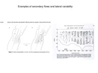
Examples of secondary flows and lateral variability. S 4. S 4. S 3. S 3. S 2. U+ D U. U- D U. U+ D U. U- D U. U- D U. U- D U. S 2. S 1. S 1. Differential Advection in channel with deep middle and Shallow flanks Producing along channel salinity gradient. Fresh. Fresh. Salty.

E N D
S4 S4 S3 S3 S2 U+DU U-DU U+DU U-DU U-DU U-DU S2 S1 S1 Differential Advection in channel with deep middle and Shallow flanks Producing along channel salinity gradient
Fresh Fresh Salty Effects of Differential Advection on Flood Tide Nunes and Simpson (1985) What’s the effect on stratification? What’s the effect on the along channel momentum balance? What happens on Ebb?
Requires Secondary flows to balance forcing Kalkwijk and Booij (1986) Geyer (1993) Pressure gradient centrifugal acceleration
Secondary flows due to flow curvature From Geyer (1993)
Baroclinic balance arrests lateral flows Chant and Wilson (1997) Seim and Gregg (1997) Pressure gradient centrifugal acceleration
Chant and Wilson, 1997 Current Vectors Upper layer Lower layer NY NJ CTD section CTD section NY NJ
ADCP mooring NOAA/NOS - PORTS mooring data. Average ebb-dry period Secondary circulation Average ebb-wet period No secondary circulation Red - Surface Blue -Middle Purple- Bottom Current Vectors
1 m/s 1 m/s Dry Period 1.5 m 1m 2 m Tidal Range Wet Period Currents during Maximum ebb Wet Period Red Surface Blue Bottom Wet Period 1.5 m 1m 2 m
Depth Depth Tidal Range Tidal Range Along Channel Flow Max Ebb vs. Tidal Range Dry Period Cross Channel Flow
Along Channel Flow NeapTides Depth Depth Cross Channel Flow Springtides Tidal Range Tidal Range Max Ebb vs. Tidal Range Wet Period
Wet Period - Maximum Ebb binned vs Tidal Range Stronger shear in along channel flow but weaker cross channel flows.
Strong Moderate Weak Complex Lateral Sloshing?? Stratification Tidal Range
Secondary flows driven by Coriolis (Lerczak and Geyer, 2004)
Az=22*10-4 m2/s Uf=0.25 cm/s Max(V)=10 cm/s Az=3.3*10-4 m2/s Uf=7.0 cm/s Max(V)= 2.6 cm/s
As stratification increases Secondary flows decrease Flood-ebb asymmetry in Secondary flows V~1/DS(z) g ranges from 1 for weakly Stratified case and approaces 100 during strongly case (represents ratio of isopycnal tilting To differential advection) Lerczak and Geyer (2004)
Tidally mean vuy+wuz Is dominated by flood Tide. Note where velocity max Is on flood (red line)
Figure 4 Salt section along Hudson during moderate to high flow condition during spring tide (upper panel) and neap tide (Lower panel). See figure 2 for timing of transects relative to river flow and tidal range
April May June Figure 5. (upper panel) along channel currents averaged between 1.35 and 6.1 meters above the bottom water from site 4 (blue line) and its low passed filtered component (green line). (lower panel) surface (green line) and bottom (blue line) salinity during the spring of 2002.
Exchange flow drops off more slowly than H&R predicts because H&R neglected the effect of lateral circulation that becomes more Important as mixing increases.
Including Coriolis produces lateral asymmetries. This would tend to transport Sediment to the right (looking seaward) and thus produce a laterally asymmetric Channel such as the Hudson.
Channel Cross-section at mooring array 1 2 3 4 Laterally Asymmetric Channel in Hudson In the afternoon we’ll look at aspects of lateral circulation based On data from the Hudson
Laterally Sheared James Neap James Spring Hudson Neap Hudson Spring Vertically Sheared Figure 3) Schematic showing movement of Hudson and James river estuary through Kevlin/Ekman number space over the spring neap cycle. Laterally sheared estuaries lie in the upper right quadrant, while vertically sheared estuaries lie in the lower left quadrant
U2,V2 U1,V1 s1s s2s s1b Full mooring deployment (Lerczak et al. 2006) and locations of Data used in afternoon experiment