Download
1 / 26
270 likes | 414 Vues
Measures of Centrality and Variability. STA 220 - Lecture #4. Centrality and Variability. Methods to take large amounts of data and present it in a concise form Want to present height of females and males in STA 220 Could measure everyone and graph results

E N D
Measures of Centrality and Variability STA 220 - Lecture #4
Centrality and Variability • Methods to take large amounts of data and present it in a concise form • Want to present height of females and males in STA 220 • Could measure everyone and graph results • More interested in that describes the most likely representation of the height of the students in the class • This is called
Centrality and Variability • Once you have your measure of centrality may want or need to know • Is the data repeatable? • This would be
Measures of Centrality • 3 common measures of centrality
Measures of Centrality • Mean • Mathematical average of all the data
Measures of Centrality • Example • Suppose Suzy is taking Chemistry. There is a lab quiz every other week. Near the end of the semester, Suzy wants to determine her quiz average. Her quiz scores are: 78, 92, 83, 95, 98, 87 and 93.
Measures of Centrality • Mathematical shorthand: • Data points are often referred to as xi where i is 1…n, n being • For Suzy’s quiz scores, n = 7 and x1 = 78, x2 = 92, x3 = 83, x4 = 95, x5 = 98, x6 = 87, and x7 = 93. • The mean would be denoted by , called x-bar. • For Suzy’s quizzes,
Measures of Centrality • The median is the of the dataset, such that half of all data points are to that value AND half of all data points are to that value.
Measures of Centrality • To find the median: • Rearrange data from smallest to largest • If n is odd, calculate • If n is even, calculate • Count the sorted data set until you get to the data point in the position you calculated in part 2 or 3 • If the number of data points, n, was odd, then you are done. If n is even, then compute the mean of the data point in the position and position.
Measures of Centrality • Example • Given the following salary information from a group of engineers, determine the median salary: $75,400; $83,600; $45,700; $43,900; $62,100; $90,500; $55,800. • First reorder the data in increasing order: • 43,900; 45,700; 55,800; 62,100; 75,400; 83,600; 90,500 • Since n = 7 is odd, compute • = (7+1)/2 = 4 • 43,900; 45,700; 55,800; ; 75,400; 83,600; 90,500
Measures of Centrality • Example • A group of students are taking the following number of credit hours: 12, 17, 15, 14, 9, 16, 18, 16, 14, 12. Find the median number of credit hours being taken by this group of students. • Put the data in increasing order: • 9, 12, 12, 14, 14, 15, 16, 16, 17, 18 • Since n = 10 is even, compute • = 10/2 = 5 • Next, identify the data points in the fifth and sixth position • 9, 12, 12, 14, 14, 15, 16, 16, 17, 18 • Compute the mean of the fifth and sixth data points • =14.5
Measures of Centrality • The mode is the number that appears the most often in the data set. • Example: Here are the number of cavities found in a class of 1st graders: • 0,1,0,1,0,5,5,3,4,0,0,2,0,1,0,3,2,4,7,1. Find the mode. • 0 occurs times, while 1 occurs times, 2, 3, 4, and 5 occurs , and 7 occurs once. As 0 occurs the most often, it is .
Measures of Centrality • Comparing Mean, Median, Mode • Mean • Strong Points • Uses all of the data • Weak Points • Sensitive to extremes. Test scores: 34, 92, 95, 94, 89 have a mean of 80.8. If the professor dropped the lowest test score, 34, then the mean would be • May not be an actual, observable value. For example, the average family has 1.6 children. What does it mean to have 0.6 of a child?
Measures of Centrality • Comparing Mean, Median and Mode • Median and Mode • Strong Points • Not sensitive to . In test score example from before the median would be 34, 89, 92, 94, 95. • The mode is an observable value; the median is an observable value • Weak Points • The value may not be unique. In the case of the mode, it is possible to have several values that appear the most. • Both do not use actual/all data values. The mode keys in on frequency, while the median just looks at the middle of the data set.
Measures of Centrality • In 1995, the mean salary of a MLB player was $1,080,000 while the median salary of a MLB player was $275,000. • Recall the median is the point where half of the data points are above and half are below – Thus, at least half of the players in the MLB earned less than • A mean of $1,080,000 tells you that there are players earning millions of dollars – but this may not be the number of all players in the MLB
Measures of Centrality • The Corps of Engineers wants to dredge a harbor in Hackensack, NJ. The EPA has these guidelines for harbor dredging: • The sediment is tested for the presence of PCBs. • If PCBs < 25 parts per billion, then its OK to dredge and dump. • If 25 ppb ≤ PCBs ≤ 50 ppb, then its OK to dredge and dump, but then a cap must be placed on the dump pile. • If PCBs ≥ 50 ppb, then the harbor can not be dredged and dumped.
Measures of Centrality • 6 samples are taken, and the average PCBs was 46.5 ppb. The Corps of Engineers should be allowed to dredge and dump the harbor, then cap the dump site…or should they? • The actual samples were: 66, 74, 81, 55, 1, 2. • The average is • The median is
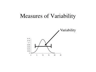
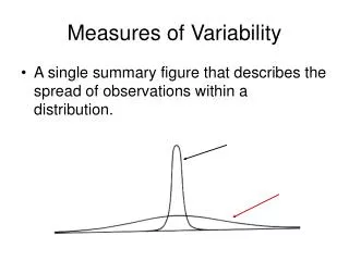
Measures of Variability • Measures of variability describe the of the data • All measures of variability are greater than or equal to • Measures close to indicate that the data is highly consistent and repeatable • 4 measures of variability: , Average deviation, , Standard Deviation
Measures of Variability • Range • Difference between the largest data point in the dataset and the smallest data point in the dataset • or Range = • Example • Suppose the daily low temperatures for the past week have been -3, -7, -2, 0, 2, 4. What is the range? • Range = = 11
Measures of Variability • Average Deviation • The average deviation of the data from its mean value. • There are 4 steps: • Compute the of the data set, x-bar • Calculate the absolute value of the between each data point, xi , and the mean value, x-bar • Add up all of the values calculated in step 2 • Divide the sum from step 3 by
Measures of Variability • Average Deviation, Example • Suppose you have the following four data points in your dataset: 1,2,4,5. Find the average deviation.
Measures of Variability • Average Deviation • In mathematical shorthand, the average deviation can be expressed as: • Good method is to make a table:
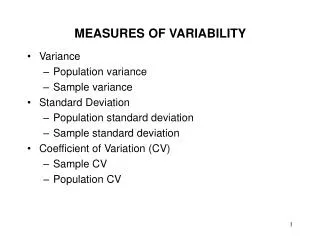
Measures of Variability • Variance • Similar to average deviation • Compute the mean of the dataset, x-bar • Calculate the difference between each data point, xi , and the mean value, x-bar • all of the values in step 2 • Add up all the values in step 3 • Divide the sum in step 4 by the total number of data points
Measures of Variability • Variance, Example • Good idea to make a table similar to the one we used for average deviation
Measures of Variability • Variance • Mathematical shorthand:
Measures of Variability • Standard Deviation • The standard deviation is just the • By taking the square root, the units of the standard deviation are the same as the original units of the data • In the previous example: