Download
1 / 33
880 likes | 5.18k Vues
Measures of Variability. In addition to knowing where the center of the distribution is, it is often helpful to know the degree to which individual values cluster around the center. This is known as variability . Range.

E N D
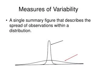
Measures of Variability • In addition to knowing where the center of the distribution is, it is often helpful to know the degree to which individual values cluster around the center. • This is known as variability.
Range • There are various measures of variability, the most straightforward being the range of the sample: Highest value minus lowest value • While range provides a good first pass at variance, it is not the best measure because of its sensitivity to extreme scores
While range provides a good first pass at variance, it is not the best measure because: • It is calculated from only 2 points of data • Those two values are the most extreme in the sample (obviously sensitive to outliers) • Can change dramatically from sample to sample
Interquartile Range • Range based on percentiles. Data can be ordered and then, much like we did for the median as the 50th percentile also known as the second quartile or Q2, we now look for numbers corresponding to the 25th and 75th percentile (Q1 and Q3). Q3- Q1 gives us the interquartile range. • Note that by only concerning oneself this middle 50% of scores, extreme scores will not affect this measure of variability. On the other hand, we also lose half our data in its calculation.
IQR and SIQR • The semi-interquartile range is simply half the IQR • Represents the average spread of those scores falling in the quartile above and below the median • If we had a scale whose median was 20 and SIQR of 5, we can say that the typical deviation of scores about the median does not extend more than 5 points above or below. • However: what if our data is skewed?
IQR: Graphical Representation • Box and whisker plots (Tukey) are graphical representations of IQR • “Hinges” mark the interquartile range • “Whiskers” encompassing 99% of the data • Any outliers designated in some fashion
The Average Deviation • Another approach to estimating variance is to directly measure the degree to which individual data points differ from the mean and then average those deviations. • That is:
The Average Deviation (cont.) • However, if we try to do this with real data, the result will always be zero: Example: (2,3,3,4,4,6,6,12)
Average Deviation • One way to get around the problem with the average deviation is to use the absolute value of the differences, instead of the differences themselves. • The absolute value of some number is just the number without any sign: For Example: |-3| = 3
Average Deviation • Thus, we could re-write and solve our average deviation question as follows: • The data set in question has a mean of 5 and a mean absolute deviation of 2.25.
The Variance • Although the MAD is an acceptable measure of variability, the most commonly used measure is variance (denoted s2 for a sample and 2 for a population) and its square root termed the standard deviation (denoted s for a sample and for a population).
The Variance (cont.) • The computation of variance is also based on the basic notion of the average deviation however, instead of getting around the “zero problem” by using absolute deviations (as in MAD), the “zero problem” is eliminating by squaring the differences from the mean. Specifically:
Variance is not too meaningful on its own. What we’d like is something that’s on the same scale as the original variable. • Standard deviation is just the square root of the variance, and gets our measure of variability back to the original scale units.
An equivalent formula that is easier to work with when calculating variances by hand is: • Although this second formula may look more intimidating, a few examples will show you that it is actually easier to work with.
Relation of range to s • If the variable is normally distributed, a rule of thumb is that: s = R/6 • This will be more clear when we talk about the normal distribution and its properties, but the idea is that roughly 99% of the data falls between 3 SD above and below the mean.
Comparing variability The coefficient of variation allows us to compare variability on measures of different scales. Often we want something that has enough variability to accurately reflect the nature of the underlying variable. Suppose someone came up with a measure of say, motivation, that was measured with questionnaire items with Likert scales ranged from 1-4. Someone else comes up with a better one that utilizes a 7 point scale. We could use the CV to compare their relative spread.
Visualizing Means and Standard Deviations This demonstration allows you to play with the mean and standard deviation of a distribution. Note that changing the mean of the distribution simply moves the entire distribution to the left or right without changing its shape. In contrast, changing the standard deviation alters the spread of the data but does not affect where the distribution is “centered” Run demo
Your turn • Find the mean, range and standard deviation of the following scores: • 3 1 7 9 8 8 5 7 4
Your turn • Mean = 5.78 • Range = 8 • s = 2.68
Estimating Population Parameters • The mean (X) and variance (s2) are the descriptive statistics that are most commonly used to represent the data points of some sample. • The real reason that they are the preferred measures of central tendency and variance is because of certain properties they have as estimators of their corresponding population parameters; and 2.
Estimating Population Parameters (cont.) • Four properties are considered desirable in a population estimator; sufficiency, unbiasedness, efficiency, & resistance. • Both the mean and the variance are the best estimators in their class in terms of the first three of these four properties. • To understand these properties, you first need to understand a concept in statistics called the sampling distribution
Sampling Distribution Demo • We will discuss sampling distributions off and on throughout the course, and I only want to touch on the notion now. • Basically, the idea is this – in order to exam the properties of a statistic we often want to take repeated samples from some population of data and calculate the relevant statistic on each sample. We can then look at the distribution of the statistic across these samples and ask a variety of questions about it. • Check out this demonstration
Properties of a Statistic • 1) Sufficiency A sufficient statistic is one that makes use of all of the information in the sample to estimate its corresponding parameter. For example, this property makes the mean more attractive as a measure of central tendency compared to the mode or median.
Estimating Population Parameters • 2) Unbiasedness A statistic is said to be an unbiased estimator if its expected value (i.e., the mean of a number of sample means) is equal to the population parameter it is estimating. Explanation of N-1 in s2 formula.
Assessing the Bias of an Estimator • Using the procedure, the mean can be shown to be an unbiased estimator. • However, if the more intuitive formula for s2 is used: • it turns out to underestimate 2
Assessing the Bias of an Estimator (cont.) • This bias to underestimate is caused by the act of sampling and it can be shown that this bias can be eliminated if N-1 is used in the denominator instead of N. • Note that this is only true when calculating s2, if you have a measurable population and you want to calculate 2, you use N in the denominator, not N-1.
Degrees of Freedom • The mean of 6, 8, & 10 = 8. • If I allow you to change as many of these numbers as you want BUT the mean must stay 8, how many of the numbers are you free to vary?
Degrees of Freedom • The point of this exercise is that when the mean is fixed, it removes a degree of freedom from your sample -- this is like actually subtracting 1 from the number of observations in your sample. • It is for exactly this reason that we use N-1 in the denominator when we calculate s2 (i.e., the calculation requires that the mean be fixed first which effectively removes -- fixes -- one of the data points).
Estimating Population Parameters • 3) Efficiency The efficiency of a statistic is reflected in the variance that is observed when one examines the statistic over a bunch of independently chosen samples. The smaller the variance, the more efficient the statistic is said to be.
Estimating Population Parameters • 4) Resistance The resistance of an estimator refers to the degree to which that estimate is effected by extreme values. As mentioned previously, both X and s2 are highly sensitive to extreme values.
Estimating Population Parameters • 4) Resistance Despite this, they are still the most commonly used estimates of the corresponding population parameters, mostly because of their superiority over other measures in terms sufficiency, unbiasedness, & efficiency.