Download
1 / 27
280 likes | 476 Vues
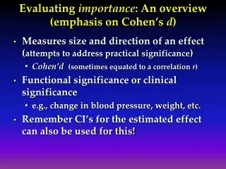
Evaluating importance : An overview (emphasis on Cohen’s d ). Measures size and direction of an effect ( attempts to address practical significance ) Cohen’d (sometimes equated to a correlation r ) Functional significance or clinical significance

E N D
Evaluating importance: An overview(emphasis on Cohen’s d) • Measures size and direction of an effect (attempts to address practical significance) • Cohen’d(sometimes equated to a correlation r) • Functional significance or clinical significance • e.g., change in blood pressure, weight, etc. • Remember CI’s for the estimated effect can also be used for this!
Practical vs statistical significance • Statistical significance (alpha level; p-value) reflects the odds that a particular finding could have occurred by chance. • If the p-value for a difference between two groups is 0.05, it would be expected to occur by chance just 5 times out of 100 (thus, it is likely to be a “real” difference). • If the p-value for the difference is 0.01, it would be expected to occur by chance just one time out of 100 (thus, we can be even more confident that the difference is real rather than random).
Practical significance • Reflects the magnitude, or size, of the difference, not the probability that the observed result could have happened by chance. • Arguably much more important than statistical significance, especially for clinical questions • Measures of effect size (ES) quantify practical significance of a finding
Effect size • The degree to which the null hypothesis is false, e.g., not just that two groups differ significantly, but how much they differ (Cohen, 1990) • Several measures of ES exist; use “whatever conveys the magnitude of the phenomenon of interest appropriate to the research context” (Cohen, 1990, p. 1310) • IQ and height example (Cohen, 1990)
The height-IQ correlation: Cohen’s (1990) example on statistical and practical significance • A study of 14,000 children ages 6-17 showed a “highly significant” (p < .001) correlation of r = .11) between height and IQ • What does this p indicate? • What’s the magnitude of this correlation? • Accounts for 1% of the variance • Based on an r this big, you’d expect that increasing a child’s height by 4 feet would increase IQ by 30 points, and that increasing IQ by 233 points would increase height by 4 inches (as a correlation, the predicted relationship could work in either direction)
2 main types of ES measures • Variance accounted for • a squared metric reflecting the percentage of variance in the dependent variable explained by the independent variable • e.g., squared correlations, odds ratios, kappa statistics • Standardized difference • scales measurements across studies into a single metric referenced to some standard deviation • d the most common and the easiest conceptually: our focus today
Effect size • APA (2001) Publication Manual mandates: . . .it is almost always necessary to include some index of effect size or strength of relationship…provide the reader not only with information about statistical significance but also with enough information to assess the magnitude of the observed effect or relationship (pp. 25-26).
APA guidelines (2001) mandate inclusion of ES information (not just p-value information) in all published reports. • Until that happy day, if ES information is missing, readers must estimate ES for themselves. • When group means and SDs are reported, you often can estimate effect size quickly and decide whether to keep reading or not.
Finding, estimating, & interpreting d in group comparison studies • d = Difference between the means of the two groups, divided by the standard deviation (SD). • Interpret as size of group difference in SDunits. • When average mean difference between tx and control groups is 0.8 to 1 SD, practical significance has been defined as “high”.
Estimating d • Find group means, subtract them, and divide by the standard deviation. • When SDs for the groups are identical, hooray. When not, arguments have been made for using the control group SD, or the average of the two SDs. • My preference is the second, which is more conservative and strikes me as more appropriate when dealing with the large variability we see in many groups of patients with disorders
Exercise 1: Calculating effect size, given group means and SDs • Data from Arnold et al. (2004) study comparing scores on SNAP composite test after four types of treatment for ADHD (Scores on SNAP composite; lower = better): Treatment group Mean (SD) Combined 0.92 (0.50) Medical management 0.95 (0.51) Behavioral 1.34 (0.56) Community care 1.40 (0.54) http://www.minddisorders.com/Kau-Nu/Kaufman-Short-Neurological-Assessment-Procedure.html (Link to the SNAP Assessment)
d demonstration, comparing SNAP performance in Combined and Medical Management groups Combined 0.92 (0.50) Medical management 0.95 (0.51) d = 0.92-0.95/0.505 = -.03/.505 = -.0594 Interpretation: The Combined group scored about 6/100s of a standard deviation better (lower) than the Medical Mgt group (an extremely tiny difference; these treatment approaches resulted in virtually the same outcomes on the SNAP measure)
d for Combined vs. Community Care treatment groups Combined 0.92 (0.50) Community care 1.40 (0.54) d = 0.92-1.40/0.52 = -0.48/.52 = -0.92 Interpretation: The Combined group scored nearly a whole standard deviation better than the Community care group; this is a large effect size. Combined treatment is substantially better than Community care.
d for Medical Management vs. Behavioral treatment Medical management 0.95 (0.51) Behavioral 1.34 (0.56) d = ? Interpretation? Assuming equal sample sizes the pooled variance is average of the sample variances, from which we can calculate the pooled SD estimate (spooled). d = (1.34 - .95)/.536 = .39/.536 = .728
d for Medical Management vs. Behavioral treatment Medical management 0.95 (0.51) Behavioral 1.34 (0.56) d = 0.95-1.34= -.39/.535 = -.72897 = -.73: Interpretation: The Medical Mgt group scored about 3/4s of a SD better than the behavioral group. This is a solid effect size suggesting that Medical Mgt treatment was substantially more effective than Behavioral treatment.
Exercise 1: Interpreting d in the happy cases when it’s reported • Treatment-difference effect sizes (Cohen’s d) from Arnold et al., 2004 (Table II, p. 45) Combined vsMedical Management 0.06 Combined vs Behavioral 0.79 Combined vs Community Care 0.92 Medical Management vs Behavioral 0.728 Medical Mgtvs Community Care 0.85 Behavioral vs Community Care 0.11 • Note that our calculated d’s match these.
An Overview of Evaluating Precision • Precision is reflected by the width of the confidence interval (CI) surrounding a given finding • Any given finding is acknowledged to be an estimate of the “real” or “true” finding • CI reflects the range of values that includes the real finding with a known probability • A finding with a narrower CI is more precise (and thus more clinically useful) than a finding with a broader CI • The standard error (SE) is the key.
Evaluating Precision • CI’s are calculated by adding and subtracting a multiple of the standard error (SE) for a finding/value (e.g., estimate +1.96xSE(estimate) to determine the 95% CI) • As we have seen the standard error depends on sample size and reliability/variability; larger samples and higher reliability (smaller variability) will result in narrower CIs, all else being equal.
Finding and interpreting evidence of precision • CI’s for difference between means of 206 children receiving early TTP and 196 receiving late TTP for OME (Paradise et al. 2001) Early Late 95% CI PPVT 92 (13) 92 (15) -2.8 to 2.8 NDW 124 (32) 126 (30) -7.6 to 4.8 PCC-R 85 (7) 86 (7) -2.1 to 0.7 • CI’s are narrow thanks to large sample
Contrast with risk estimates for low PCC-R from smaller samples of children with (n=15) and without (n=47) OME-associated hearing loss. (Shriberget al., 2000) • Estimated risk was 9.60 (i.e., children with hearing loss were 9.6 times more likely to have low PCC-R at age 3 than children without. • But 95% confidence interval was 1.08-85.58 – meaning that this increased risk was somewhere between none and a lot. Not very precise!
Predict precision • In one study, children with histories of OME (n=10) had significantly lower scores on a competitive listening task than children without OME histories (n=13) OME+ OME- p -6.8 (2.8) -9.7 (2.6) .016 • How could you quantify importance? • What would you predict about precision?
When multiple studies of a question are available, meta-analysis • Quantitative summary of effects across a number of studies addressing particular question, usually in the form of a d (effect size) statistic • In EBP evidence reviews, the highest quality evidence comes from meta-analysis of studies with strong validity, precision, and importance
A meta-analysis of OME and speech and language (Casby, 2001) • Casby (2001) summarized results of available studies of OME and children’s language. • For global language abilities, the effect size for comparing mean language scores from children with and without OME histories was d = -.07. • Interpretation and a graphic representation.
An informative graphic for meta-analyses • Shows d from each study as well as associated 95% CI.
dand 95% CI boundaries for OME and vocabulary comprehension (Casby, 2001) Study Paradise 00 Black 93 Lonigan 92 Roberts 91m Upper 95% CI d Roberts 91l Lower 5% CI Teele 90 Lous 88 Teele 84 2.5 -2.5 -2 -1.5 -1 -0.5 0 0.5 1 1.5 2 Better with OME Worse with OME Overall d = .001
Evidence levels for evaluating quality of treatment studies Best Ia Meta-analysis of >1 randomized controlled trial (RCT) Ib Well-designed randomized controlled study IIa Well-designed controlled study without randomization IIb Well-designed quasi-experimental study III Well-designed non-experimental studies, i.e., comparative, correlational, and case studies Worst IV Expert committee report, consensus conference, clinical experience of respected authorities
Summary of Effect Size Cohen’s d can be “equated” to a correlation. Provides a standardized measure of effect size. Best way to discern practical significance from statistical significance is direct quantification of effect size using a CI. For meta-analysis however, we need a standardized ES in order to combine study results.