Growth and Output
320 likes | 699 Vues
Growth and Output. Econ 102. Countries: High savings rate have higher GDP/ cap. high population growth rates have low GDP/ cap. . Solow model: . Solow model: . Solow model with increase in savings rate: . Solow model with improvement in technology : . Output grows over time:.

Growth and Output
E N D
Presentation Transcript
Growth and Output Econ 102
Countries: • High savings rate have higher GDP/ cap. • high population growth rates have low GDP/ cap.
Which output level is produced: Demand and Supply Aggregate Demand and Aggregate Supply
SR and LR Aggregate Supply • There are constraints on Price changes and Output changes. • Short run AS : price pressures are less, there are unemployed resources and if demand increases output increase without price increase. • Long run AS: capacity of production is constant, an increase in demand increases prices but not quantity. • Very long run: capacity is growing, shifts in the LRAS curve.
SR and LR Aggregate Supply SR Aggregate Supply LR Aggregate Supply
Aggregate Demand • Total of desired aggregate expenditures • Which type expenditures? • Desired Consumption Expenditures: • Desired Investment Expenditures: • Government Expenditures: • Net Exports:
WHY ‘DESIRED’ EXPENDITURES? • Agents may want to purchase, may plan to buy but Are there enough goods there? If not ? What happens? How does the adjustment occur? What happened at the end of 2008 in Turkey?
‘Desired’ Aggregate Expenditures • Buyers in the Goods Market and Services Market: • Desired Consumption Expenditures, • Desired Investment Expenditures, • Desired Government Expenditures, • Desired Net Exports WHY ‘DESIRED’ EXPENDITURES?
What determines the desired AE? • AEd= Cd + Id + Gd + Xd – Md • Household: Cd depends on Disposable Income. • Firms: Id depends on cost of borrowing. • External Sector: Xd and Md depends on exchange rate and Income. • Government: determines its own expenditure level Gd (it is a policy tool).
When will there be an equilibrium? • When aggregate desired expenditures are equal to total output produced AEd = Y • If Aggregate demand is less than output AEd < Y stocks of unsold good will be used. • If Aggregate demand is more than output Aed < Y stocks of unsold good will pile up.
Equilibrium in a Macroeconomy • Graphical Presentation and Equilibrium:
Disequilibrium adjustment • If the economy starts at a point where AE≠Y; what happens? The forces in the economy will bring the economy to the equilibrium output level. (Stable equilibrium) If for example AE<Y… then inventories will pile up, the firms will cancel orders, firms will cut back production, fire workers, employment and production will decline until AE=Y. (Reverse is also true for AE>Y )
Equilibrium in a Macroeconomy Keynesian Model: (emphasizes the demand side) • If AEd > Y , then there is unplanned decline in the inventory levels of the firms, firms start to increase production. • If AEd=Y , then there is no unplanned change in inventory levels,no change in production (Equilibrium). • If AEd < Y , then there is unplanned increase in the inventory levels of the firms, firms start to decrease production.
A Model for Desired Aggregate Expenditures • Desired Consumption Expenditures: Cd • What is DisposableIncome? YD • Thereforedesiredconsumptionexpendituresare an increasingfunction of Y.
A Model for Desired Aggregate Expenditures • Desired Investment Expenditures: Id • Therefore we can write as:
A Model for Desired Aggregate Expenditures • Desired Government Expenditures: Gd • Therefore we can write as:
A Model for Desired Aggregate Expenditures • Desired Net Exports: NXd (in the simple model) • Therefore we can write as:
Mathematical Example • Steps to find the Equilibrium Income (Output): • Find Desired Aggregate Expenditure Function as a function of Y. • Use equilibrium condition: AEd= Y • Solve for Y, which will be the level of output which is equal to the level of AEd. Example…
Why does the Equilibrium Income change? • If any of the autonomous spending increase then equilibrium income will increase from YE to YENEW. • Possible causes of autonomous income increase are: • (Graphically all of these are vertical (upward) shift of the AE function)
How does the Equilibrium Income change? Example: If Investment increases from to (where ) Then
How does Eq. Income respond to a change in AEd? • What is the change in equilibrium income if Id increases? • ( ) • Multiplier: Numeric example…
Why is there a ‘multiplier effect’? • Initial increase in autonomous spending sets off a series of increase in AE and in real GDP. • First increases, which means firms want to purchase purchase more new machines, the AE in the economy increases, the factories which makes these machines will hire workers. This will increase their salary payments, the workers will increase their desired consumption and hence the economy will move to a higher Y level along the new AE function.