Download
1 / 18
180 likes | 210 Vues
This study explores internal wave generation over the continental shelf using analytical and numerical approaches, assessing model limitations and comparing results with an idealized case.

E N D
Internal Tide Generation Over a Continental Shelf Summer 2008 internship Gaёlle Faivre Flavien Gouillon, Alexandra Bozec Pr. Eric P. Chassignet
Biography • Gaëlle Faivre • Student from the Engineering School in Mathematic Modeling and Mechanics (MATMECA) • Bordeaux, FRANCE • Position at COAPS: • Internship from June 2 - Sept 16, 2008
Outline • Introduction • Motivation • Objective • Approach • - Analytical solution • - Numerical experiment • Results • Conclusion
I. Introduction • Internal waves review: • Internal waves occur in stably stratified fluids when a water parcel is displaced by some external force and is restored by buoyancy forces. Then the restoration motion may overshoot the equilibrium position and set up an oscillation thereby forming an internal wave. • Internal tide comes from the interaction between rough topography and the barotropic tide. • Important internal wave generation occurs at the shelf break where the slope is abrupt. • - Horizontal length scales of the order 1 to 100 km • - Horizontal Velocity of 0.05 to 0.5 m.s-1 • - Time scale of minutes to days
Surface signature of an internal wave An example of a surface signature of an internal wave View from a boat
II. Motivation • Knowledge of internal wave generation and how they propagate is crucial to understand ocean mixing and the large scale ocean circulation. • Internal waves generation at the shelf affects: • sediment transport • biology • oil production companies • submarine navigation. • At the shelf, the dynamic of internal wave is strongly non-hydrostatic and thus cannot be well resolved in Oceanic General Circulation Models that usually make the hydrostatic approximation
III. Objectives • Assess the HYbrid Coordinate Ocean Model (HYCOM) skills to simulate internal wave at an abrupt slope. • Evaluate and document the limitation of HYCOM on representing these waves.
IV. Approach Compute an analytical solution for an idealized case of internal tide generation over a shelf break Build the same configuration with HYCOM Compare the dynamical properties as well as the energetic of the generated internal wave for both results.
Analytical solution Conditions for this analytic results: - The flow is two-dimensional - 2 layers ocean - The interface between the 2 layers needs to be smaller than the shelf depth • Based on Griffiths and Grimshaw, (2004) • There is one baroclinic mode with the phase speed: Figure 1: schematic of the analytical model Dimensions : • Wave speed at the shelf • Wave speed in the deep ocean :
Pulsation: Frequency: Analytical energy computation The nondimensional depth-integrated energy fluxes at the shelf are given by: JL Semi-diurnal frequency: Steepness parameter: Prediction of the low energy flux • Change in phase across the slope is given by: • Low energy fluxes located each , where the slope accommodates an integer number of wavelengths of the internal wave • High energy fluxes located each
HYCOM • HYCOM is run in fully isopycnal mode for this configuration. • We used all the same parameters as the analytical configuration and vary the steepness parameter by changing the stratification, and the interface depth but keeping a constant shelf length/coast length ratio (Ls/Lc). • Objectives: Show that low energy fluxes are simulated in HYCOM and well located when Ls/Lc=1. Schematic of the Model Configuration Analytical Energy Fluxes
Results: Energy fluxes comparison • Energy fluxes as a function of the steepness parameter (function of the wave speed at the shelf) for HYCOM Analytical Solution Energy fluxes (W.m-2) Low energy fluxes expected at
Discussion • We obtain low energy fluxes just like the analytical solution predicted. However some of them seem to be not located correctly for a particular choice of parameters. • What could cause this shift in the low energy location? • Not enough sampling (because each point is a different configuration) • Several approximations and truncations are made in the internal wave group speed and in the internal wave energy computations • HYCOM does not represent the wave propagation correctly (wavelength, wave speed)
Conclusion • We have found an analytical solution for the internal wave generation at a shelf with a 2-layers ocean idealized problem. • We have conducted numerical simulations with HYCOM for the same configuration. • Low energy fluxes are represented in HYCOM. • For a particular choice of parameters, these some of the low energy fluxes seems to be shifted from where the analytical solution predicts. • This could be due to our mistakes or HYCOM errors on the representing the propagation of the waves
Future Work • More simulations should be run in order to analyze the origin of the shift in the low energy fluxes • From the small scale of s1? • Computational errors in model? • Human errors? • Further analyses of the approximations in our computations should be made • Additional model configurations • Observe climatological density stratifications and adapt it to realistic continental shelves. • Examine the effects of alongshore variability in shelf topography (application to 3 dimensions) • Include nonlinear and nonhydrostatic terms
c = L 0 . 8 c R Interface displacement of the internal waves Fig2:Displacement of the interface for a horizontal normalization Fig3: Internal tide of two-layer fluid, with , at
Baroclinic zonal velocities Snapshot after 45 hours, (right after spin-up) Velocity (ms-1) The interface displacement is about 1 meter and compares well with the analytical prediction (difficult to see displacement from the scale of the figure)


![The European North Atlantic shelf [Ocean-Shelf Exchange, internal waves]](https://cdn0.slideserve.com/118374/the-european-north-atlantic-shelf-ocean-shelf-exchange-internal-waves-dt.jpg)