Stability
Stability. References: - “ Applied Nonlinear Control”, J-J. E. Slotine, W. Li, Prentice-Hall, 1991 - “Control of Robot Manipulators”, F.L. Lewis, C.T. Abdallah, D.M. Dawson, Macmillan, 1993 .


Stability
E N D
Presentation Transcript
References: - “ Applied Nonlinear Control”, J-J. E. Slotine, W. Li, Prentice-Hall, 1991 - “Control of Robot Manipulators”, F.L. Lewis, C.T. Abdallah, D.M. Dawson, Macmillan, 1993
DefinitionThe equilibrium point 0 is stable if for any R>0 , there exists a positive scalar r(R, t0 ) such that Otherwise, the equilibrium point 0 is unstable. ex) Instability of the Van der Pol oscillator The Van der Pol oscillator is described by One easily shows that the system has an equilibrium point at the origin. curve 1-asymptotically stable curve 2-marginally stable (stable in the sense of Lyapunov) curve 3-unstable
Definition An equilibrium point 0 is exponentially stable if there exist two strictly positive numbers and ,such that for sufficient small is some ball Br around the origin. • DefinitionThe equilibrium point at the origin is asymptotically stable at time t0 if • It is stable
ex) The system is exponentially convergent to x =0 with a rate . Indeed, its solution is and therefore Note : 1) Exponential stability implies asymptotic stability. 2) Asymptotic stability does not guarantee exponential stability, as can be seen from the system whose solution is x=1/(1+t), a function slower than any exponential function
Definition If asymptotic (or exponential) stability holds for any initial states, the equilibrium point is said to be asymptotically (or exponentially) stable in the large. It is also called globally asymptotically (or exponentially) stable. DefinitionThe equilibrium point 0 is locally uniformly stable if the scalar r in the previous definition of stability can be chosen independently of t0, i.e., if r = r(R).
DefinitionThe equilibrium point at the origin is locally uniformly asymptotically stable if • It is uniformly stable • There exists a ball of attraction BRo , whose radius is independent of t0 , such that any system trajectory with initial states in BRo converges to 0 uniformly in t0 By uniform convergence in terms of , we mean that for all and satisfying , such that, , i.e., the state trajectory, starting from within a ball BR1, will converge into a smaller ball BR2 after a time period T which is independent of t0.
ex) Consider the first-order system This system has the general solution This solution asymptotically converges to zero. But the convergence is not uniform. Intuitively, this is because a larger t0 requires a longer time to get close to the origin.
Definition A scalar continuous function V(x) is said to be locally positive definite if V(0) = 0 and, in a ball BRo If V(0) = 0 and the above property holds over the whole state space, then V(x) is said to be globally positive definite.
DefinitionIf, in a ball BRo, the function V(x) is positive definite and has continuous partial derivatives, and if its time derivative along any state trajectory of system is negative semi-definite, i.e., then V(x) is said to be a Lyapunov function for the system.
Theorem (Local Stability)If, in a ball BRo, there exists a scalar function V(x) with continuous first partial derivatives such that • is positive definite (locally in BRo ) • is negative semi-definite (locally in BRo) then the equilibrium point 0is stable. If, actually, the derivative is locally negative definite in BRo , then the stability is asymptotic. Theorem (Global Stability)Assume that there exists a scalar function V of the state x, with continuous first order derivatives such that • is positive definite • is negative definite • as then the equilibrium at the origin is globally asymptotically stable.
Notes: 1) Asymptotic stability is a very important property to be determined. It only holds when the derivative of the Lyapunov function is negative definite in equilibrium point theorems . 2) In some situations, even the derivative of the Lyapunov function is still negative semi-definite, it is possible to draw conclusions on asymptotic stability with help of the powerful invariant set theorem attributed by La Salle. 3) The invariant set theorem is a generalization of the concept of equilibrium point theorem.
DefinitionA set G is an invariant set for a dynamic system if every system trajectory which originates from a point in G remains in G for all future time. ex) equilibrium point, limit cycle, whole state space(trivial one) Theorem (Local Invariant Set Theorem) Consider an autonomous system of the form , with f continuous, and let V(x) be a scalar function with continuous first partial derivatives. Assume that for some l > 0, the region l defined by Let R be the set of all points within l where and M be the largest invariant set in R. Then, every solution x(t) originating in l tends to M ast
DefinitionA transfer function h(p) is positive real if It is strictly positive real if h(p-) is positive real for some > 0. TheoremA transfer function h(p) is strictly positive real (SPR) if and only if i) h(p) is a strictly stable transfer function ii) the real part of h(p) is strictly positive along the j axis, i.e.,
ex) SPR and non-SPR transfer functions Consider the following systems The transfer functions h1, h2, and h3 are not SPR, because h1 is non-minimum phase, h2 is unstable, and h3 has relative degree larger than 1.
Is the (strictly stable, minimum-phase, and of relative degree 1) function h4 actually SPR? We have (where the second equality is obtained by multiplying numerator and denominator by the complex conjugate of the denominator) and thus which shows that h4 is SPR (since it is also strictly stable).
TheoremA transfer function h(p) is positive real if, and only if, i) h(p) is a stable transfer function. ii) The poles of h(p) on the axis are simple (i.e., distinct) and the associated residues are real and non-negative. iii) Re[h(j)] 0 for any 0 such that is not a pole of h(p). Lemma(Kalman-Yakubovitch) Consider a controllable linear time-invariant system The transfer function is strictly positive real if, and only if, there exist positive definite matrices P and Q such that
Lemma(Meyer-Kalman-Yakubovitch)Given a scalar vector b and c, an asymptotically stable matrix A, and a symmetric positive definite matrix L, if the transfer function is SPR, then there exist a scalar , a vector q, and a symmetric positive definite matrix P such that This lemma is different from Positive Real Lemma (KY Lemma ) in two aspects. First, the involved system now has the output equation Second, the system is only required to be stabilizable (but not necessarily controllable).
DefinitionAn m x m transfer function matrix H(p) is called PR if H(p) has elements which are analytic for Re(p)>0; H(p) + HT(p*) is positive semi-definite for Re(p)>0. where the asterisk * denotes the complex conjugate transpose. ex)
Definition H is Lp stable if Hu belongs to whenever u belongs to and there exists finite constants and b such that If p = , the system is said to be bounded-input/bounded-output (BIBO) stable. DefinitionThe Lp gain of the system H is denoted by and is the smallest such that a finite b exists to verify the equation
H(·) Passive Systems DefinitionConsider the system shown in the figure, and assume that it has the same number of inputs and outputs [i.e., u(t) and y(t) have the same dimension]. Passivity: The system is said to be passive if for all finite T > 0 . Strict Passivity: The system is said to be strictly passive if there for all finite T > 0.
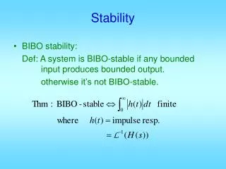
H1 Theorem : (Small-Gain Theorem) Let H1: and H2: . Therefore, H1 and H2 satisfy the inequalities for all T [0,) and suppose . If then and . H2
Notes: Basically, the small-gain theorem states that a feedback interconnection of two systems is BIBO stable if the loop gain is less than unity. A passive system is in effect one that does not create energy. If the system under consideration is linear and time invariant, then passivity is equivalent to positivity and may be tested in the frequency domain.