Download
1 / 30
300 likes | 411 Vues
This workshop explores the integration of downscaling techniques within hydrological models to assess climate change impacts on water resources. Attendees will learn about the bias correction processes for GCM simulations, the significance of selecting appropriate emissions scenarios, and the use of downscaled data to inform water management strategies. By analyzing various future scenarios and utilizing probabilistic projections, participants will enhance their ability to adapt water resources planning to climate variability and extreme weather events.

E N D
Downscaling for the World of Water E.P. Maurer Santa Clara University, Civil Engineering Dept. NCPP Workshop Quantitative Evaluation of Downscaling 12-16 August, 2013 Boulder, CO
Estimating Climate Impacts to Water 2. Global Climate Model 4. Land surface (Hydrology) Model 1. GHG Emissions Scenario 5. Operations/impacts Models • “Downscaling” Adapted from Cayan and Knowles, SCRIPPS/USGS, 2003
Downscaling: bringing global signals to regional scale GCM scale and processes at too coarse a scale Figure: Wilks, 1995 • Resolved by: • Bias Correction • Spatial Downscaling
IPCC CMIP3 GCM Simulations • 20th century through 2100 and beyond • >20 GCMs • Multiple Future Emissions Scenarios http://www-pcmdi.llnl.gov/
2/3 chance that loss will be at least 40% by mid century, 70% by end of century Point at: 120ºW, 38ºN Impact Probabilities for Planning Snow water equivalent on April 1, mm • Combine many future scenarios, models, since we don’t know which path we’ll follow (22 futures here) • Choose appropriate level of risk
Incorporating probabilistic projections into water planning • Overdesign for present • Can represent declining return periods for extreme events Das et al, 2012 Mailhot and Sophie Duchesne, JWRPM, 2010
Monthly downscaled data • PCMDI CMIP3 archive of global projections • 16 GCMs, 3 Emissions • 112 GCM runs • Allows quick analysis of multi-model ensembles • gdo4.ucllnl.org/downscaled_cmip3_projections
Use of U.S. Data Archive • Thousands of users downloaded >20 TB of data • Uses for Research (R), Management & Planning (MP), Education (E)
Downscaling for Extreme Events • Some impacts due to changes at short time scales • Heat waves • Flood events • Daily GCM output limited for CMIP3, more plentiful for CMIP5 • Downscaling adapted for modeling extremes
Archive expansion • Daily downscaled data (BCCA) • Hydrology model output • CMIP5
Online Analysis and Download withhttp://ClimateWizard.org • Global and US data sets • Country and US state boundaries defined • Spatial and time series analysis • Ensemble quick view • Upload of custom shapefiles Girvetz et al., PLoS, 2009
Information Overload (practitioner’s dilemma) • Little guidance in selection of: • Emissions • GCMs • Downscaling methods • Hundreds of downscaled GCM runs • Many impacts studies cannot use all of them • How much information is really useful?
Selecting 4 Specific GCM Runs • Bivariate probability plot shows correlation between T, P • Identify Change Range: 10 to 90 %-tile T, P • Select bounds based on: • risk attitude • interest in breadth of changes • number of simulations desired Brekke et al., 2009
Selecting GCMs for Impact Studies • Ensemble mean provides better skill • Little advantage to weighting GCMs according to skill • Most important to have “ensembles of runs with enough realizations to reduce the effects of natural internal climate variability” [Pierce et al., 2009] • Maybe 10-14 GCMs is enough? Gleckler, Taylor, and Doutriaux, Journal of Geophysical Research (2008) as adapted by B. Santer Brekke et al., 2008
Discard CMIP3 in favor of CMIP5? • Ensemble average changes comparable • RCP8.5 and SRES A2 comparable
Is BCSD method valid? • At each grid cell for “training” period, develop monthly CDFs of P, T for • GCM • Observations (aggregated to GCM scale) • Obs are from Maurer et al. [2002] • Use quantile mapping to ensure monthly statistics (at GCM scale) match obs • Apply same quantile mapping to “projected” period Wood et al., BAMS 2006
Are biases time-invariant? Biases vary in time, space, at quantiles R index: compares size of bias variability to average GCM bias
Time-invariant enough… • On average, time-invariant enough where bias correction works • But for small ensembles maybe not (locations where biases vary with time differ for GCMs)
Bias correction changes trends! Raw GCM Bias Corrected • Changes in mean annual precipitation: 1970-1999 to 2040-2069 • Similar effect in CMIP3 and CMIP5 • Some more intense wettening in Rockies for CMIP5
What happens? • Contrived Example (Precipitation): • Gamma distributions • asymmetry • Obs: mean=30 • GCM Historic has −30% bias in SD • GCM future has +40% change in mean
What is effect of trend/shift? • Quantile mapping changes shift in mean • +40% becomes +56% • -40% becomes -39% • 5% decrease changes to ~2% increase
But is changing the trend bad? • estimated change in precip from 1916-1945 and 1976-2005. • Where index is >1 BC worsens • Ensemble avg shows trend modification not consistently bad. Ensemble Avg
Challenges in providing downscaled data for water-resources community • With >500 projections at 1 archive (of many), need to provide users with better information for: • Selecting concentration pathways • Assembling an ensemble of GCMs • Using data downscaled appropriately • Interpreting results with uncertainty • Despite known issues with every step, useful information can produced by this process. • Bottom line for data users: Use an ensemble. Don’t worry. Revisions happen.
A1B Scenario Source: Girvetz et al, PloS, 2009 Global BCSD • Similar to US archive, but ½-degree • Publicly available since 2009 • Captures variability among GCMs • www.engr.scu.edu/~emaurer/global_data/ • Data accessed by users in all 50 States and 99 countries (11 months only)