Download
1 / 51
510 likes | 933 Vues
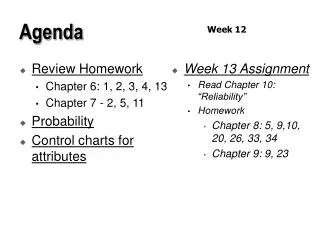
Agenda. Week 12. Review Homework Chapter 6: 1, 2, 3, 4, 13 Chapter 7 - 2, 5, 11 Probability Control charts for attributes. Week 13 Assignment Read Chapter 10: “Reliability” Homework Chapter 8: 5, 9,10, 20, 26, 33, 34 Chapter 9: 9, 23. Probability . Chapter Eight.

E N D
Agenda Week 12 • Review Homework • Chapter 6: 1, 2, 3, 4, 13 • Chapter 7 - 2, 5, 11 • Probability • Control charts for attributes • Week 13 Assignment • Read Chapter 10: “Reliability” • Homework • Chapter 8: 5, 9,10, 20, 26, 33, 34 • Chapter 9: 9, 23
Probability Chapter Eight Probability
Probability theorems • Probability is expressed as a number between 0 and 1 • Sum of the probabilities of the events of a situation equals 1 • If P(A) is the probability that an event will occur, then the probability the event will not occur is • 1.0 - P(A) Probability
Probability theorems • For mutually exclusive events, the probability that either event A or event B will occur is the the sum of their respective probabilities. • When events A and B are not mutually exclusive events, the probability that either event A or event B will occur is • P(A or B or both) = P(A) + P(B) - P(both) Probability
Probability theorems • If A and B are dependent events, the probability that both A and B will occur is • P(A and B) = P(A) x P(B|A) • If A and B are independent events, then the probability that both A and B will occur is • P(A and B) = P(A) x P(B) Probability
Permutations and combinations • A permutation is the number of arrangements that n objects can have when r of them are used. • When the order in which the items are used is not important, the number of possibilities can be calculated by using the formula for a combination. Probability
Discrete probability distributions • Hypergeometric - random samples from small lot sizes. • Population must be finite • samples must be taken randomly without replacement • Binomial - categorizes “success” and “failure” trials • Poisson - quantifies the count of discrete events. Probability
Continuous probability distributions • Normal • Uniform • Exponential • Chi Square • F • student t Probability
Fundamental concepts • Probability = occurrences/trials • 0 < P < 1 • The sum of the simple probabilities for all possible outcomes must equal 1 • Complementary rule - P(A) + P(A’) = 1 Probability
Addition rule • P(A + B) = P(A) + P(B) - P(A and B) • If mutually exclusive; just P(A) + P(B) P(AandB) P(A) P(B) Probability
Addition rule example • P(A + B) = P(A) + P(B) - P(A and B) • Roll one die • Probability of even and divisible by 1.5? • Sample space {1,2,3,4,5,6} • Event A - Even {2,4,6} • Event B - Divisible by 1.5 {3,6} • Event A and B ? • Solution? Probability
Conditional probability rule • P(A|B) = P(A and B) / P(B) • A die is thrown and the result is known to be an even number. What is the probability that this number is divisible by 1.5? • P(/1.5|Even)=P(/1.5 and even)/P(even) • 1/6 / 3/6 = 1/3 Probability
Compound or joint probability • The probability of the simultaneous occurrence of two or more events is called the compound probability or, synonymously, the joint probability. • Mutually exclusive events cannot be independent unless one of them is zero. Probability
Multiplication for independent events • P(A and B) = P(A) x P(B) • P(ace and heart) = P(ace) x P(heart) • 1/13 x 1/4 = 1/52 Probability
Computing conditional probabilities • P(A|B) = P(A and B)/P(B) • P(Own and Less than 2 years)? Probability
Computing conditional probabilities • P(A|B) = P(A and B)/P(B) P(AandB) P(A) P(B) Probability
Conditional probability Satisfied Not Satisfied Totals New 300 100 400 Used 450 150 600 Total 750 250 1000 S=satisfied N= bought new car P(N|S) = ? Probability
60 business students from a large university are surveyed with the following results: 19 read Business Week 18 read WSJ 50 read Fortune 13 read BW and WSJ 11 read WSJ and Fortune 13 read BW and Fortune 9 read all three How many read none? How many read only Fortune? How many read BW, the WSJ, but not Fortune? Hint: Try a Venn diagram. Just for fun Probability
Probability Distributions Probability
Learning objectives • Know the difference between discrete and continuous random variables. • Provide examples of discrete and continuous probability distributions. • Calculate expected values and variances. • Use the normal distribution table. Probability
Random variables • A random variable is a numerical quantity whose value is determined by chance. • “A random variable assigns a number to every possible outcome or event in an experiment”. • For non-numerical outcomes such as a coin flip you must assign a random variable that associates each outcome with a unique real number. Probability
Random variable types • Discrete random variable - assumes a limited set of values; non-continuous, generally countable • number of Mark McGwire homeruns in a season • number of auto parts passing assembly-line inspection • GRE exam scores Probability
Random variable types • Continuous random variable - random variable with an infinite set of values. 0.000 Baseball player’s batting average 1.000 Can occur anywhere on a continuous number scale Probability
Random variables and probability distributions • The relationship between a random variable’s values and their probabilities is summarized by its probability distribution. Probability
Probability distribution • Whether continuous or discrete, the probability distribution provides a probability for each possible value of a random variable, and follows these rules: • The events are mutually exclusive • The individual probability values are between 0 and 1. • The total value of the probability values sum to 1 Probability
Possible rate of return 10% 11% 12% 13% 14% 15% 16% 17% Probability .05 .15 .20 .35 .10 .10 .03 .02 Total = 1.0 Probability distribution for rates of return Probability
Measures of central tendency expected value (weighted average) Measures of variability variance standard deviation Describing distributions Probability
Expected value of a discrete random variable • For discrete random variables, the expected value is the sum of all the possible outcomes times the probability that they occur. E(X) = {xi * P(xi)} Probability
Example: A fair die • Roll 1 die: x P(x) x*P(x) E(x)=? 1 1/6 1/6 2 1/6 2/6 3 1/6 3/6 4 1/6 4/6 5 1/6 5/6 6 1/6 6/6 Can you sketch the distribution? Probability
Fair die illustrates a discrete “uniform distribution” • The random variable, x, has n possible outcomes and each outcome is equally likely. Thus, x is distributed uniform. Probability
Probability distribution P(x) 1/6 x 1 2 3 4 5 6 Probability
Example: An unfair die • Roll 1 die: x P(x) x*P(x) E(x)=? 1 1/12 1/12 2 2/12 4/12 3 2/12 6/12 4 2/12 8/12 5 2/12 10/12 6 3/12 18/12 Can you sketch the distribution? Probability
Expected value of a bet • Suppose I offer you the following wager: You roll 1 die. If the result is even, I pay you $2.00. Otherwise you pay me $1.00. • E(your winnings)=.5 ($2.00) + .5 (-1.00) = 1.00 - .50 = $0.50 Probability
Expected Value of a Bet • Suppose I offer you the following wager: You roll 1 die. If the result is 5 or 6 I pay you $3.00. Otherwise you pay me $2.00. • What is your expected value? Probability
Variance of a discrete random variable The variance of a random variable is a measure of dispersion calculated by squaring the differences between the expected value and each random variable and multiplying by its associated probability. {(xi-E(x))2 * P(xi)} Probability
Example: A fair die • Roll 1 die: [x- E(X)] 2 P(x) *P(x) 1 - 21/6 6.25 1/6 1.04 2 - 21/6 2.25 1/6 .375 3 - 21/6 .25 1/6 .04 4 - 21/6 .25 1/6 .04 5 - 21/6 2.25 1/6 .375 6 - 21/6 6.25 1/6 1.04 2.91 Probability
Probability distributions for continuous random variables • A continuous mathematical function describes the probability distribution. • It’s called the probability density function and designated ƒ(x) • Some well know continuous probability density functions: • Normal Beta • Exponential Student t Probability
Continuous probability density function - Uniform If a random variable, x, is distributed uniform over the interval [a,b], then its pdf is given by 1 b-a a b Probability
Uniform What is the probability of x? 1 b-a x a b Probability
Uniform Area under the rectangle = base*height = (b-a)* 1 = 1 b-a 1 b-a a b Probability
Uniform P(c<x<b) = Area of brown rectangle 1 * (b-c) Ht x Width) = b-a 1 b-a c a b Probability
Uniform P(2<x<5) = Brown rectangle 1 * (5-2) =(1/4) *3 =3/4 = 5-1 1 5-1 =1/4 2 1 5 Probability
Uniform distribution If a random variable, x, is distributed uniform over the interval [a,b], then its pdf is given by And, the mean and variance are (a+b) ( b-a )2 E(x) = ------- Var(x)=--------- 2 12 Probability
Uniform Mean? Variance? 3 8 Probability
Calculate uniform mean, variance So, if a = 3 and b = 8 And, the mean and variance are (a+b) ( b-a )2 25 E(x) = ------ = 5.5 V(x)=--------- = ----- = 2.08 2 12 12 Probability
Continuous pdf - Normal If x is a normally distributed variable, then is the pdf for x. The expected value is and the variance is 2. Probability
One standard deviation 68.3% Probability
Two standard deviations 2 2 95.5% Probability
Three standard deviations 3 3 99.73% Probability