Download
1 / 52
530 likes | 685 Vues
This lecture explores exemplary inverse problems, focusing on techniques such as thermal diffusion and earthquake location. It covers the methodology for solving inverse problems using principles like the Backus-Gilbert theory and damped least squares. The discussion includes the resolution trade-offs when reconstructing initial conditions from measurements over time, particularly in the context of thermal diffusion in cooling slabs and seismic wave analysis. Students will learn about the application of generalized inverses and the importance of measurement accuracy in deriving meaningful solutions.

E N D
Lecture 23 Exemplary Inverse ProblemsincludingEarthquake Location
Syllabus Lecture 01 Describing Inverse ProblemsLecture 02 Probability and Measurement Error, Part 1Lecture 03 Probability and Measurement Error, Part 2 Lecture 04 The L2 Norm and Simple Least SquaresLecture 05 A Priori Information and Weighted Least SquaredLecture 06 Resolution and Generalized Inverses Lecture 07 Backus-Gilbert Inverse and the Trade Off of Resolution and VarianceLecture 08 The Principle of Maximum LikelihoodLecture 09 Inexact TheoriesLecture 10 Nonuniqueness and Localized AveragesLecture 11 Vector Spaces and Singular Value Decomposition Lecture 12 Equality and Inequality ConstraintsLecture 13 L1 , L∞ Norm Problems and Linear ProgrammingLecture 14 Nonlinear Problems: Grid and Monte Carlo Searches Lecture 15 Nonlinear Problems: Newton’s Method Lecture 16 Nonlinear Problems: Simulated Annealing and Bootstrap Confidence Intervals Lecture 17 Factor AnalysisLecture 18 Varimax Factors, Empircal Orthogonal FunctionsLecture 19 Backus-Gilbert Theory for Continuous Problems; Radon’s ProblemLecture 20 Linear Operators and Their AdjointsLecture 21 Fréchet DerivativesLecture 22 Exemplary Inverse Problems, incl. Filter DesignLecture 23 Exemplary Inverse Problems, incl. Earthquake LocationLecture 24 Exemplary Inverse Problems, incl. Vibrational Problems
Purpose of the Lecture • solve a few exemplary inverse problems • thermal diffusion • earthquake location • fitting of spectral peaks
Part 1 • thermal diffusion
0 temperature in a cooling slab h x ξ 1.0 erf(x) 0.5 0.0 1 2 3 x
temperature due to M cooling slabs (use linear superposition)
temperature due to M slabs each with initial temperature mj temperature measured at time t>0 initial temperature
inverse problem infer initial temperature m using temperatures measures at a suite of xs at some fixed later time t data model parameters d = G m
distance, x 0 100 -100 0 time, t temperature, T 200
distance, x 0 100 -100 0 initial temperature consists of 5 oscillations time, t 200
distance, x 0 100 -100 0 time, t oscillations still visible so accurate reconstruction possible 200
distance, x 0 100 -100 0 time, t 200 little detail left, so reconstruction will lack resolution
What Method ? The resolution is likely to be rather poor, especially when data are collected at later times damped least squares G-g = [GTG+ε2I]-1GT damped minimum length G-g = GT [GGT+ε2I]-1 Backus-Gilbert
What Method ? The resolution is likely to be rather poor, especially when data are collected at later times damped least squares G-g = [GTG+ε2I]-1GT damped minimum length G-g = GT [GGT+ε2I]-1 Backus-Gilbert actually, these generalized inverses are equal
What Method ? The resolution is likely to be rather poor, especially when data are collected at later times damped least squares G-g = [GTG+ε2I]-1GT damped minimum length G-g = GT [GGT+ε2I]-1 Backus-Gilbert might produce solutions with fewer artifacts
Try both damped least squares Backus-Gilbert
Solution Possibilities • Damped Least Squares: Matrix G is not sparse no analytic version of GTG is available M=100 is rather small experiment with values of ε2 mest=(G’*G+e2*eye(M,M))\(G’*d) 2. Backus-Gilbert use standard formulation, with damping α experiment with values of α
Solution Possibilities • Damped Least Squares: Matrix G is not sparse no analytic version of GTG is available M=100 is rather small experiment with values of ε2 mest=(G’*G+e2*eye(M,M))\(G’*d) 2. Backus-Gilbert use standard formulation, with damping α experiment with values of α try both
estimated initial temperature distributionas a function of the time of observation True Damped LS Backus-Gilbert time time time distance distance distance
estimated initial temperature distributionas a function of the time of observation True Damped LS Backus-Gilbert time time time distance distance distance Damped LS does better at earlier times
estimated initial temperature distributionas a function of the time of observation True Damped LS Backus-Gilbert time time time distance distance distance Damped LS contains worse artifacts at later times
model resolution matrix when for data collected at t=10 Damped LS Backus-Gilbert distance distance distance distance
model resolution matrix when for data collected at t=10 Damped LS Backus-Gilbert distance distance distance distance resolution is similar
Damped LS Backus-Gilbert model resolution matrix when for data collected at t=40 distance distance distance distance
Damped LS Backus-Gilbert model resolution matrix when for data collected at t=40 distance distance distance distance Damped LS has much worse sidelobes
Part 2 • earthquake location
ray approximation vibrations travel from source to receiver along curved rays r x S s P z
ray approximation vibrations travel from source to receiver along curved rays r x S s P z S wave slower P wave faster P, S ray paths not necessarily the same, but usually similar
travel time T integral of slowness along ray path r x S s P z TS = ∫ray (1/vS) d𝓁 TP = ∫ray (1/vP) d𝓁
arrival time = travel time along ray + origin time data data earthquake location 3 model parameters earthquake origin time 1 model parameter
arrival time = travel time along ray + origin time explicit nonlinear equation 4 model parameters up to 2 data per station
arrival time = travel time along ray + origin time linearize around trial source location x(p) • tiP = TiP(x(p),x(i)) + [∇TiP] • ∆x + t0 trick is computing this gradient
Geiger’s principle r r ray x(1) Δx x(1) x(0) Δx x(0) • [∇TiP] = -s/v unit vector parallel to ray pointing away from receiver
Common circumstances when earthquake far from stations All rays leave source at the same angle x z All rays leave source at nearly the same angle x z
then, if only P wave data is available (no S waves) these two columns are proportional to one-another
depth and origin time trade off x z deep and late shallow and early
Solution Possibilities • Damped Least Squares: Matrix G is not sparse no analytic version of GTG is available M=4 is tiny experiment with values of ε2 mest=(G’*G+e2*eye(M,M))\(G’*d) 2. Singular Value Decomposition to detect case of depth and origin time trading off test case has earthquakes “inside of array”
z, km y, km x, km
Part 3 • fitting of spectral peaks
1 0.95 0.9 0.85 0.8 0.75 0.7 0.65 0 2 4 6 8 10 12 typical spectrum consisting of overlapping peaks xx counts counts counts velocity, mm/s velocity, mm/s
what shape are the peaks? try both use F test to test whether one is better than the other
what shape are the peaks? 3 unknowns per peak data data 3 unknowns per peak both cases: explicit nonlinear problem
issueshow to determinenumber q of peakstrial Aicifiof each peak
our solutionhave operator click mouse computer screento indicate position of each peak
MatLab code for graphical input K=0; for k = [1:20] p = ginput(1); if( p(1) < 0 ) break; end K=K+1; a(K) = p(2)-A; v0(K)=p(1); c(K)=0.1; end