Download
1 / 61
640 likes | 1.01k Vues
Inventory Management, Just-in-Time, and Backflush Costing. JOIN KHALID AZIZ. ECONOMICS OF ICMAP, ICAP, MA-ECONOMICS, B.COM. FINANCIAL ACCOUNTING OF ICMAP STAGE 1,3,4 ICAP MODULE B, B.COM, BBA, MBA & PIPFA. COST ACCOUNTING OF ICMAP STAGE 2,3 ICAP MODULE D, BBA, MBA & PIPFA. CONTACT:

E N D
JOIN KHALID AZIZ • ECONOMICS OF ICMAP, ICAP, MA-ECONOMICS, B.COM. • FINANCIAL ACCOUNTING OF ICMAP STAGE 1,3,4 ICAP MODULE B, B.COM, BBA, MBA & PIPFA. • COST ACCOUNTING OF ICMAP STAGE 2,3 ICAP MODULE D, BBA, MBA & PIPFA. • CONTACT: • 0322-3385752 • 0312-2302870 • R-1173,ALNOOR SOCIETY, BLOCK 19,F.B.AREA, KARACHI, PAKISTAN.
JOIN KHALID AZIZ • FRESH CLASSES • ICMAP STAGE 1 & 2 • FUNDAMENTALS OF FINANCIAL ACCOUNTING & COST ACCOUNTING • INDIVIDUAL & GROUPS
Learning Objective 1 Identify five categories of costs associated with goods for sale.
Costs Associated withGoods for Sale 1. Purchasing costsinclude transportation costs. 2. Ordering costs include receiving and inspecting the items in the orders. 3. Carrying costs include the opportunity cost of the investment tied up in inventory and the costs associated with storage.
Costs Associated withGoods for Sale 4. Stockout costs occur when an organization runs out of a particular item for which there is a customer demand. 5. Quality costsof a product or service is its lack of conformance with a prespecified standard.
Learning Objective 2 Balance ordering costs with carrying costs using the economic-order-quantity (EOQ) decision model.
Economic-Order-QuantityDecision Model Assumptions 1. The same quantity is ordered at each reorder point. 2. Demand, ordering costs, carrying costs, and purchase-order lead time are known with certainty. 3. Purchasing costs per unit are unaffected by the quantity ordered.
Economic-Order-QuantityDecision Model Assumptions 4. No stockouts occur. 5. Quality costs are considered only to the extent that these costs affect ordering costs or carrying costs.
Economic-Order-QuantityDecision Model Assumptions The EOQ minimizes the relevant ordering costs and carrying costs. Video store sells packages of blank video tapes. Video purchases packages of video tapes from Oaks, Inc., at Rs.15/package.
Economic-Order-QuantityDecision Model Assumptions Annual demand is 12,844 packages, at the rate of 247 packages per week. Video requires a 15% annual return on investment. The purchase-order lead time is two weeks. What is the economic-order-quantity?
Economic-Order-QuantityDecision Model Assumptions Relevant ordering cost per purchase order: Rs.209 Relevant carrying costs per package per year: Required annual ROI (15% × Rs.15) Rs.2.25 Relevant other costs 3.25 Total Rs.5.50
Economic-Order-Quantity Decision Model Example EOQ = D = Demand in units for a specified time period P = Relevant ordering costs per purchase order C = Relevant carrying costs of one unit in stock for the time period used for D
Economic-Order-Quantity Decision Model Example EOQ = = 988 packages
Economic-Order-Quantity Decision Model Example What are the relevant total costs (RTC)? RTC = Annual relevant ordering costs + Annual relevant carrying costs RTC = D Q × P + Q 2 × C DP Q + QC 2 or Q can be any order quantity, not just the EOQ.
Economic-Order-Quantity Decision Model Example When Q = 988 units, RTC = (12,844 × Rs.209 ÷ 988) + (988 × Rs.5.50 ÷ 2) = Rs.5,434 total relevant costs How many deliveries should occur each time period? D EOQ = 12,844 988 = 13 deliveries
JOIN KHALID AZIZ • FRESH CLASSES • MA-ECONOMICS • MICRO, Macro & STATISTICS • INDIVIDUAL & GROUPS
Economic-Order-Quantity Decision Model Example 10,000 8,000 Annual relevant total costs Relevant Total Costs (Dollars) 6,000 5,434 Annual relevant ordering costs 4,000 Annual relevant carrying costs 2,000 600 988 EOQ 1,200 1,800 2,400 Order Quantity (Units) 20 - 15
Reorder Point Reorder point = Number of units sold per unit of time × Purchase-order lead time EOQ = 988 packages Number of units sold/week = 247 Purchase-order lead time = 2 weeks Reorder point = 247 × 2 = 494 packages
Reorder Point 988 Reorder Point Reorder Point 494 Weeks 1 2 3 4 5 6 7 8 Lead Time 2 weeks Lead Time 2 weeks This exhibit assumes that demand and purchase-order lead time are certain: Demand = 247 tape packages/week Purchase-order lead time = 2 weeks 20 - 17
Safety Stock Example Safety stock is inventory held at all times regardless of the quantity of inventory ordered using the EOQ model. Video’s expected demand is 247 packages per week. Management feels that a maximum demand of 350 packages per week may occur.
Safety Stock Example How much safety stock should be carried? 350 Maximum demand – 247 Expected demand = 103 Excess demand per week 103 packages × 2 weeks lead time = 206 packages of safety stock.
Considerations in ObtainingEstimates of Relevant Costs What are the relevant incremental costs of carrying inventory? – only those costs of the purchasing company that change with the quantity of inventory held
Cost of Prediction Error Predicting relevant costs requires care and is difficult. Assume that Video’s relevant ordering cost is Rs.97.84 instead of the Rs.209 prediction used. What is the cost of this prediction error?
Cost of Prediction Error Step 1: Compute the monetary outcome from the best action that could have been taken, given the actual amount of the cost input. EOQ = EOQ = = 676 packages
Cost of Prediction Error The annual relevant total costs when EOQ is 676 packages is: RTC = DP Q + QC 2 RTC = (12,844 × Rs.97.84 ÷ 676) + (676 × Rs.5.50 ÷ 2) = Rs.3,718 total relevant costs
Cost of Prediction Error Step 2: Compute the monetary outcome from the best action based on the incorrect amount of the predicted cost input. EOQ = = 988 packages
Cost of Prediction Error What are the annual relevant costs using this order quantity when D = 12,844 units, P = Rs.97.84, and C = Rs.5.50? RTC = (12,844 × Rs.97.84 ÷ 988) + (988 × Rs.5.50 ÷ 2) = Rs. 3,989 total relevant costs
Cost of Prediction Error Step 3: Compute the differencebetween the monetary outcomes from Steps 1 & 2. Step 1 Rs.3,718 Step 2 3,989 Difference Rs. (271) The cost of prediction error is Rs.271.
Learning Objective 3 Identify and reduce conflicts that can arise between EOQ decision model and models used for performance evaluation.
Evaluating Managers andGoal-Congruence Issues The opportunity cost of investment tied up in inventory is a key input in the EOQ decision model. Some companies now include opportunity costs as well as actual costs when evaluating managers.
Just-In-Time Purchasing Just-in-time (JIT) purchasing is the purchase of goods or materials such that a delivery immediately precedes demand or use. Companies moving toward JIT purchasing argue that the cost of carrying inventories (parameter C in the EOQ model) has been dramatically underestimated in the past.
JIT Purchasing and EOQModel Parameters The cost of placing a purchase order (parameter P in the EOQ model) is also being re-evaluated. Three factors are causing sizable reduction in the cost of placing a purchase order (P). 1. Companies increasingly are establishing long-run purchasing arrangements.
JIT Purchasing and EOQModel Parameters 2. Companies are using electronic links, such as the Internet, to place purchase orders. 3. Companies are increasing the use of purchase order cards (similar to consumer credit cards like Visa and Master Card).
Learning Objective 4 Use a supply-chain approach to inventory management.
Supply-Chain Analysis Supply-chain analysis describes the flow of goods, services, and information from cradle to grave, regardless of whether those activities occur in the same organization or other organizations. “bullwhip effect” or “whiplash effect”
JOIN KHALID AZIZ • FRESH CLASSES • ICMAP STAGE 1 & 2 • FUNDAMENTALS OF FINANCIAL ACCOUNTING & COST ACCOUNTING • INDIVIDUAL & GROUPS
Learning Objective 5 Differentiate materials requirements planning (MRP) systems from just-in-time (JIT) systems for manufacturing.
Materials RequirementPlanning (MRP) Materials requirements planning (MRP) systems take a “push-through” approach that manufactures finished goods for inventory on the basis of demand forecasts. MRP predetermines the necessary outputs at each stage of production.
Materials RequirementPlanning (MRP) Management accountants play key roles in an MRP system, including... – maintaining accurate and timely information pertaining to materials, work in process, and finished goods, and... – providing estimates of the setup costs for each production run, the downtime costs, and carrying costs of inventory.
Learning Objective 6 Identify the features of a just-in-time production system.
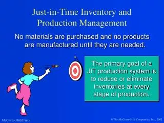
Just-In-Time Production Systems Just-in-time (JIT) production systems take a “demand pull” approach in which goods are only manufactured to satisfy customer orders.
Major Features of a JIT System 1. Organizing production in manufacturing cells 2. Hiring and retaining multi-skilled workers 3. Emphasizing total quality management 4. Reducing manufacturing lead time and setup time 5. Building strong supplier relationships
Major Features of a JIT System What information may management accountants use? Personal observation by production line workers and managers Financial performance measures, such as inventory turnover ratios Nonfinancial performance measures of time, inventory, and quality.
Learning Objective 7 Use backflush costing.
Backflush Costing Backflush costing describes a costing system that delays recording some or all of the journal entries relating to the cycle from purchase of direct materials to the sale of finished goods.
Backflush Costing Where journal entries for one or more stages in the cycle are omitted, the journal entries for a subsequent stage use normal or standard costs to work backward to flush out the costs in the cycle for which journal entries were not made.
Learning Objective 8 Describe different ways backflush costing can simplify traditional job-costing systems.
Trigger Points The term trigger point refers to a stage in a cycle going from purchase of direct materials to sale of finished goods at which journal entries are made in the accounting system.
Trigger Points Stage A: Purchase of direct materials Stage B: Production resulting in work in process Stage C: Completion of good units of product Stage D: Sale of finished goods
![]Just In Time (JIT) Inventory Management](https://cdn4.slideserve.com/7168704/slide1-dt.jpg)