Chapter 4 Statistics
Chapter 4 Statistics. 4.1 – What is Statistics?. Definition 4.1.1 Data are observed values of random variables. The field of statistics is a collection of methods for estimating distributions and parameters of random variables through the collection and analysis of data.

Chapter 4 Statistics
E N D
Presentation Transcript
4.1 – What is Statistics? Definition 4.1.1 Data are observed values of random variables. The field of statistics is a collection of methods for estimating distributions and parameters of random variables through the collection and analysis of data.
4.1 – What is Statistics? Definition 4.1.2 The population is the set of all objects of interest in a statistical study. A sample is a subset of the population. Definition 4.1.3 Data are information that has been collected. The field of statistics is a collection of methods for drawing conclusions about a population by collecting and anlyzingdata from a sample.
Types of Data Definition 4.1.4 A parameter is a number calculated using information from every member of a population. A statistic is calculated using information from a sample. Definition 4.1.5 Quantitative data consist of numbers. Qualitative data are nonnumeric information that can be separated into different categories.
Types of Data Definition 4.1.6 Discrete data are observed values of a discrete random variable. They are numbers that have a finite or countable set of values. Continuous data are observed values of a continuous random variable. They are numbers that can take any value within some range.
Levels of Measurement Definition 4.1.7 • Data are at the nominal level of measurement if they consist of only names, labels, or categories. They cannot be ordered (such as smallest to largest) in a meaningful way. • Data are at the ordinal level of measurement if they can be ordered in a meaningful way, but differences between data values cannot be calculated or are meaningless. • Data are at the interval level of measurement if they can be ordered in a meaningful way and differences between data values are meaningful. • Data are at the ratio level of measurement if they are at the interval level, ratios of data values are meaningful, and there is meaningful zero starting point.
Types of Studies Definition 4.1.8 • In an observational study, data is obtained in a way such that the members of the sample are not changed, modified, or altered in any way. • In an experiment, something is done to the members of the sample and the resulting effects are recorded. The “something” that is done is called a treatment.
Types of Observational Studies Definition 4.1.9 • In a cross-sectional study, data are collected at one specific point in time. • In a retrospective study, data are collected from studies done in the past. • In a prospective study, data are collected by observing a sample for some time into the future.
Blocks Definition 4.1.10 A block is a subset of the population with a similar characteristic. Different blocks of a population have different characteristics that may affect the variable of interest differently. A randomized block design is a type of experiment where: • The population is divided into blocks. • Members from each block are randomly chosen to receive the treatment.
Sampling Techniques Definition 4.1.11 • A convenience sample is a sample that is very easy to get. • A voluntary response sample is obtained when members of the sample decide whether to participate or not. • A systematic sample is obtained by arranging the population in some order, then selecting a starting point, and then selecting every kthmember (such as every 20th).
Sampling Techniques • A cluster sample is obtained by dividing the population into subsets (or clusters) where the members of each cluster have a common characteristic, then randomly choosing some of the clusters, and surveying every member of the chosen clusters. • A stratified sample is obtained by dividing the population into subsets and then randomly choosing some members from each of the subsets. • A multistage sample is obtained by successively applying a variety of sampling techniques. At each stage the sample becomes smaller, and at the last stage, a clustersampleis chosen.
Random Samples Definition 4.1.12 • A random sample is chosen in a way such that every individual member of the population has the same probability of being chosen. • A simple random sample of size n is chosen in a way such that every group of size n has the same probability of being chosen.
4.2 – Summarizing Data Example 4.2.3 Shown below are the waiting times of 30 customers at a supermarket check-out stand Relative frequency distribution
Histograms The “shape” of a relative frequency histogram is an approximation of the graph of the p.d.f. (or p.m.f.) of the underlying random variable.
Summary Statistics Definition 4.2.1 Let {x1, x2,…, xn}be a set of quantitative data collected from a sample of the population • mean of the data: • variance of the data: • standard deviation of the data: • range of the data: (max value) – (min value)
Percentiles Definition 4.2.2 Let p be a number between 0 and 1. The (100p)th percentile of a set of quantitative data is a number, denoted πp, that is greater than (100p)% of the data values. • The 25th, 50th, and 75thpercentiles are called the first, second and third quartiles and are denoted p1= π0.25, p2= π0.50, and p3 = π0.75, respectively. • The 50th percentile is also called the median of the data and is denoted m = p2. • The mode of the data is the data value that occurs most frequently. • The 5-number summary of a set of data consists of the minimum value, p1, p2, p3, and the maximum value.
Calculating Percentiles • Arrange the data in increasing order: • Calculate • If is not an integer, then round it up to the next larger integer and • If L is an integer, then
Example 4.2.5 • Calculate the first quartile, p1 = π0.25 • Calculate the median m = p2 = π0.5
Example 4.2.5 • 5-number summary 0, 0.5, 1.8, 2.9, 7.3 • Box Plot
4.4 – Sampling Distributions Definition 4.4.1 A random variable whose values are used to estimate the value of a parameter is called an estimator of . A value of , , is called an estimate of . An estimator is called an unbiased estimator of if If this equation is not true, then is called a biased estimator.
Sample Proportion Suppose we want to know the proportion p of a population who support a particular political candidate • p is a parameter We survey 735 voters and find 383 that support the candidate • The sample proportion is • This is an estimate of p
Sample Proportion Let denote the number who support the candidate in a sample of • Define the random variable • Called the “sample proportion” • is an observed value of • is an estimate of p • is an estimator of p
Sampling Distribution of the Proportion Theorem 4.4.1 Letbe b(n, p). Thenas the distribution of the sample proportion • Meaning: is approximately for n “large enough” • “Large enough” - and
Example 4.4.3 By examining the spending habits of one particular consumer, a credit card company observes that during the course of normal transactions 37% of the charges exceed $150. Out of 50 charges made in one particular month, 27 exceeded $150. Does it appear that these charges were made in the course of normal transactions?
Example 4.4.3 Sample prop. that exceed $150: • Is this unusually large? • Assume normal transactions: is approximately • This probability is small (< 0.05) • Reject the assumption
Sample Mean Suppose we want to know the mean IQ score of all college students in the US, • Estimate it with a sample mean • Let denote the IQ of a randomly selected student • is an observed value of the sample mean • is an estimate of • is an estimator of
Sampling Distribution of the Mean • By the Central Limit Theorem • where
4.5 – Confidence Intervals for a Proportion Definition 4.5.1 Let Z be and p be a number between 0 and 0.5. A critical z-value is a positive number such that
Critical Values Let be between 0 and 1. Then is between 0 and 0.5, so that the critical z-value is a positive number such that
Confidence Interval Definition 4.5.2 Let and let x be a number of successes in n observed trials of a Bernoulli experiment with unknown probability of a success p. Define and let be a critical z-value. The interval is called a 100(1 − α)% confidence interval estimate for p.
Confidence Interval Different forms
Requirements • The sample must be random. • The conditions for a binomial distribution must be satisfied (at least approximately). • There are at least 5 successes and at least 5 failures observed in the n trials.
Example 4.5.2 Suppose 383 out of 735 surveyed voters support a particular political candidate. Calculate a 95% confidence interval estimate for the proportion of all voters who support the candidate. • Define the population proportion being estimated: p = The proportion of all voters who support the candidate • Calculate the sample proportion
Example 4.5.2 • Find the critical value: • Calculate the margin of error • Calculate the confidence interval
Example 4.5.2 Correct interpretation • We are 95% confident that the value of p is between 0.485 and 0.557. Meaning • If we were to survey many different samples of voters and calculate the corresponding 95% confidence interval using the statistics from each sample, then about 95% of the intervals would contain the true value of p.
4.6 – Confidence Intervals for a Mean Definition 4.6.1 Let be the mean of a sample of size n taken from a population with known variance and unknown mean μ. The interval is called a 100(1 − α)% confidence interval estimate for μ.
Z-Interval Requirements • The sample is random. • The population variance is known. • The population is normally distributed or .
T-Interval Definition 4.6.2 Let be the mean and be the variance of a sample of size n taken from a population with unknown variance and mean μ, and let be a critical Student-t value with degrees of freedom. The interval is called a 100(1 − α)% confidence interval estimate for μ when is unknown.
T-Interval Requirements • The sample is random. • The population is normally distributed or n > 30.
Which Type of Interval? Suggestions • If n > 30 or is known, then use a Z-interval. • If is unknown, and the population is normally distributed (at least approximately), then use a T-interval. • If n ≤ 30, is unknown, and the population is not normally distributed, then see Chapter 7.
Example 4.6.3 A random sample of 15 “1-pound” packages of shredded cheddar cheese has a mean weight of lb. and standard deviation of s = 0.02 lb. Calculate a 99% confidence interval estimate for the mean weight of all such packages. • Define the population mean being estimated: = The mean weight of all “1-pound” packages of shredded cheddar cheese.
Example 4.6.3 • Find the critical value: α = 0.01 and n = 15 • Calculate the margin of error: • Calculate the confidence interval:
4.7 – Confidence Intervals for a Variance Definition 4.7.1 Let be the variance of a sample of size n taken from a normally distributed population with unknown variance and let be critical values. The interval is a 100(1 − α)% confidence interval estimate for .
Confidence Intervals for a Variance Requirements • The sample is random. • The population is normally distributed.
Example 4.7.2 The proportion of butterfat in 20 batches of butter were measured. The resulting data have a sample variance of . Construct a 95% confidence interval estimate of the variance in the proportion of butterfat of all batches. • Define the population variance being estimated: = The variance in the proportion of butterfat of all batches of butter
Example 4.7.2 • Find the critical values: and • Calculate the confidence interval:
4.8 – Confidence Intervals for Differences Definition 4.8.1 Consider two populations with respective proportions and . Let • and be the sample sizes • and be the sample proportions Then is a 100(1 − α)% confidence interval estimate for
2-Proportion Z-Interval Requirements • Both samples are random and independent. • Each sample contains at least 5 successes and 5 failures.
2-Sample T-Interval If two populations are (approximately) normally distributed and their variances are unknown, then an approximate 100(1 − α)% confidence interval for the difference of their means using data from two independent samples of the respective populations is