
GRAPH ALGORITHMS BASICS
E N D
Presentation Transcript
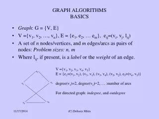
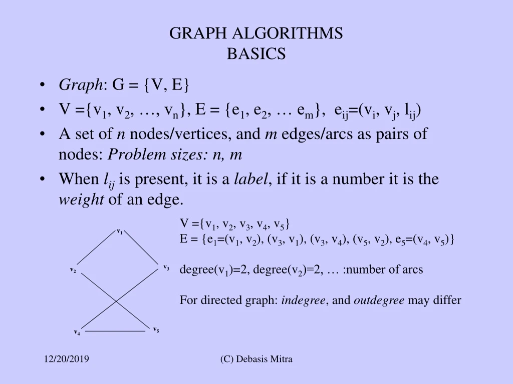
GRAPH ALGORITHMSBASICS Graph: G = {V, E} V ={v1, v2, …, vn}, E = {e1, e2, … em}, eij=(vi, vj, lij) A set of n nodes/vertices, and m edges/arcs as pairs of nodes: Problem sizes: n, m When lij is present, it is a label, if it is a number it is the weight of an edge. V ={v1, v2, v3, v4, v5} E = {e1=(v1, v2), (v3, v1), (v3, v4), (v5, v2), e5=(v4, v5)} degree(v1)=2, degree(v2)=2, … :number of arcs For directed graph: indegree, and outdegree may differ v1 v3 v2 v5 v4 (C) Debasis Mitra
GRAPH ALGORITHMSBASICS Adjacency List Representation: v1: (v2,10), (v3, 20) v2: (v1,10), (v5, 25) v3: (v1,20), (v4, 30) v4: (v3,30), (v5, 50) v5: (v2,25), (v4, 50) Weighted graph G: V ={v1, v2, v3, v4, v5} E = {(v1, v2, 10), (v3, v1, 20), (v3, v4 , 30), (v5, v2 , 25), (v4, v5 , 50)} v1 10 20 Matrix representation: v3 Matrix representation for directed Graph? v2 30 25 Matrix representation for unweighted Graph? v5 v4 50 (C) Debasis Mitra
Directed graph: edges are ordered pairs of nodes. Weighted graph: each edge (directed/undirected) has a weight. Path between a pair of nodes vi, vk: sequence of edges with vi, vk at the two ends. Simple path: covers no node in it twice. Loop: a path with the same start and end node. Path length: number of edges in it. Path weight: total wt of all edges in it. Connected graph: there exists a path between every pair of nodes, no node is disconnected. Complete graph: edge between every pair of nodes [NUMBER OF EDGES?]. Acyclic graph: a graph with no cycles. Etc. Graphs are one of the most used models of real-life problems for computer-solutions. GRAPH ALGORITHMSBASICS (C) Debasis Mitra
Algorithm 1: For each node v in V do -Steps- // (|V|) Algorithm 2: For each node v in V do For each edge in E do -Steps- // (|V|*|E|) Algorithm 3: For each node v in V do For each edge e adjacent to v do -Steps- // ( |E| ) with adjacency list, // but (|V|* |V| ) for matrix representation Algorithm 4: For each node v in V do -steps- For each edge e of v do -Steps- // ( |V|+|E| ) or ( max{|V|, |E| }) GRAPH ALGORITHMSBASICS v1 10 20 v3 v2 30 25 v5 v4 50 (C) Debasis Mitra
TOPOLOGICAL SORTProblem 1 Input: directed acyclic graph Output: sequentially order the nodes without violating any arc ordering. Note: you may have to check for cycles - depending on the problem definition (input: directed graph). An important data: indegree of each node - number of arcs coming in (#courses pre-requisite to "this" course). (C) Debasis Mitra
TOPOLOGICAL SORTProblem 1 Input: directed acyclic graph Output: sequentially order the nodes without violating any arc direction. A first-pass Algorithm: Assign indegree values to each node In each iteration: Eliminate one of the vertices with indegree=0 and its associated (outgoing) arcs (thus, reducing indegrees of the adjacent nodes) - after assigning an ordering-number (as output of topological-sort ordering) to these nodes, keep doing the last step for each of the n number-of-nodes. If at any stage before finishing the loop, there does not exist any node with indegree=0, then a cycle exists! [WHY?] A naïve way of finding a vertex with indegree0 is to scan the nodes that are still left in the graph. As the loop runs for ntimes this leads to (n2) algorithm. (C) Debasis Mitra
TOPOLOGICAL SORTProblem 1 Input: A directed graph Output: A sorting on the node without violating directions, or Failure Algorithm naïve-topological-sort 1 For each node v ϵ V calculate indegree(v); // (|E|=m) 2 counter = 0; 3 While V≠ empty do // (|V|=n) 4 find a node v ϵ V such that indegree(v) = = 0; // have to scan all nodes here: (n) // total: (n) x (while loop’s n) = O(n2) 5 if there is no such v then return(Failure) else 6 ordering-id(v) = ++counter; 7 V = V – v; 8 For each edge (v, w) ϵ E do //nodes adjacent to v //adjacent nodes: (m), total for all nodes O(n or m) 9 decrement indegree(w); 10 E = E – (v, w); end if; end while; End algorithm. Complexity: dominating term O(n2) (C) Debasis Mitra
TOPOLOGICAL SORTProblem 1 v1 Indegree(v1)=0 Indegree(v2)=1 Indegree(v3)=1 Indegree(v4)=2 Indegree(v5)=1 Ordering-id(v1) =1 Eliminate node v1, and edges (v1,v2), (v1,v3) from G Update indegrees of nodes v2 and v3 v3 v2 v5 v4 (C) Debasis Mitra
TOPOLOGICAL SORTProblem 1 Indegree(v2)=0 Indegree(v3)=0 Indegree(v4)=2 Indegree(v5)=1 Id(v1) =1, Id(v2)=2 Eliminate node v2, and edges (v2,v5) from G Update indegrees of nodes v5 v3 v2 v5 v4 (C) Debasis Mitra
TOPOLOGICAL SORTProblem 1 Indegree(v3)=0 Indegree(v4)=2 Indegree(v5)=0 Id(v1) =1, Id(v2)=2, Id(v3)=3 Eliminate node v3, and edge (v3,v4) from G Update indegrees of nodes v4 v3 v5 v4 (C) Debasis Mitra
TOPOLOGICAL SORTProblem 1 Indegree(v4)=1 Indegree(v5)=0 Id(v1) =1, Id(v2)=2, Id(v3)=3, Id(v5)=4 Eliminate node v5, and edge (v5,v4) from G Update indegrees of nodes v4 v5 v4 (C) Debasis Mitra
TOPOLOGICAL SORTProblem 1 Indegree(v4)=0 id(v1) =1, id(v2)=2, id(v3)=3, id(v5)=4, id(v4)=5 Eliminate node v4 from G, and V is empty now Resulting sort: v1, v2, v3, v5, v4 v4 (C) Debasis Mitra
TOPOLOGICAL SORTProblem 1 v1 However, now, Indegree(v1)=0 Indegree(v2)=2 Indegree(v3)=1 Indegree(v4)=2 Indegree(v5)=1 id(v1) =1 Eliminate node v1, and edges (v1,v2), (v1,v3) from G Update indegrees of nodes v2 and v3 v3 v2 v5 v4 (C) Debasis Mitra
TOPOLOGICAL SORTProblem 1 Indegree(v2)=1 Indegree(v3)=0 Indegree(v4)=2 Indegree(v5)=1 id(v1) =1, id(v3)=2 Eliminate node v3, and edge (v3,v4) from G Update indegrees of nodes v4 v3 v2 v5 v4 (C) Debasis Mitra
TOPOLOGICAL SORTProblem 1 Indegree(v2)=1 Indegree(v4)=1 Indegree(v5)=1 No node to choose before all nodes are ordered: Fail v2 v5 v4 (C) Debasis Mitra
TOPOLOGICAL SORTProblem 1 • A smarter way: notice indegrees become zero for only a subset of nodes in a pass, • but all nodes are being checked in the above naïve algorithm. • Store those nodes (who have become “roots” of the truncated graph) in a box • and pass the box to the next iteration. • An implementation of this idea may be done by using a queue: • Push those nodes whose indegrees have become 0’s (when you update those values), • at the back of a queue; • Algorithm terminates on empty queue, • but having empty Q before covering all nodes: • we have got a cycle! (C) Debasis Mitra
TOPOLOGICAL SORTProblem 1 Algorithm Q-based-topological-sort 1 For each vertex v in G do // initialization 2 calculate indegree(v); // (m)with adjacency list 3 if indegree(v) = =0 then push(Q, v); end for; 4 counter = 0; 5 While Q is not empty do // indegree becomes 0 once & only once for a node // so, each node goes to Q only once: (n) 6 v = pop(Q); 7 ordering-id(v) = ++counter; 8 V = V – v; 9 For each edge (v, w) ϵ E do //nodes adjacent to v // two loops together (max{N, |E|}) // each edge scanned once and only once 10 E = E – (v, w); 11 decrement indegree(w); 12 if now indegree(w) = =0 then push(Q, w); end for; end while; 13 if counter != N then return(Failure); // not all nodes are numbered yet, but Q is empty // cycle detected; End algorithm. Complexity: the body of the inner for-loop is executed at most once per edge, even considering the outer while loop, if adjacency list is used. The maximum queue length is n. Complexity is (m + n). (C) Debasis Mitra
SOURCE TO ALL NODES SHORTEST PATH-LENGTHProblem 2 Path length = number of edges on a path. Compute shortest path-length from a given source node to all nodes on the graph. Strategy: starting with the source as the "current-nodes," in each of the iteration expand children (adjacent nodes) of "current-nodes." Assign the iteration# as the shortest path length to each expanded node, if the value is not already assigned. Also, assign to each child, its parent node-id in this expansion tree (to retract the shortest path if necessary). Input: Undirected graph, and source node Output: Shortest path-length to each node from source This is a breadth-first traversal, nodes are expanded as increasing distances from the source: 0, then 1, then 2, etc. (C) Debasis Mitra
SOURCE TO ALL NODES SHORTEST PATH-LENGTHProblem 2 Once again, the children are pushed at the back of a queue. Input: Undirected graph, and source node Output: Shortest path-length to each node from source Algorithm q-based-shortest-path 1 d(s) = 0; // source 2 enqueue only s in Q; // (1), no loop, constant-time 3 while (Q is not empty) do // each node goes to Q once and only once: (n) 4 v = dequeueQ; 5 for each vertex w adjacent to v do // (m) 6 if d(w) is yet unassigned then // this is a graph traversal 7 d(w) = d(v) + 1; 8 last_on_path(w)= v; 9 enqueuew in Q; end if; end for; end while; End algorithm. Complexity: (m + n), by a similar analysis as that of the previous queue-based algorithm. (C) Debasis Mitra
SOURCE TO ALL NODES SHORTEST PATH-LENGTHProblem 2 Source: v1 : v1, length=0 Queue: v1 v3 v2, length=1 v3, length=1 v2 v5, length=1 Queue: v2,v3 , v5 Q: v3 ,v5 v1, no v1, no v5, already assigned v1, no v5 v1, no v4 v4, length=2 Q: v4 v3, no Q: empty (C) Debasis Mitra
SOURCE TO ALL NODES SHORTEST PATH-WEIGHT Problem 3 Input: Positive-weighted graph, a “source” node s Output: Shortest distance to all nodes from the source s v1 10 20 70 v3 v2 Breadth-first search does not work any more! Say, source is v1 Shortest-path-length(v5) = 35, not 70 However, the concept works: expanding distance front from s 25 30 v5 v4 50 (C) Debasis Mitra
SINGLE SOURCE SHORTEST PATH: Djikstra’s Algorithm Input: Weighted graph Dsw , a “source” node s [can not handle negative cycle] Output: Shortest distance to all nodes from the source s Algorithm Dijkstra 1 s.distance = 0; // shortest distance from s 2 mark s as “finished”; //shortest distance to s from s found 3 For each node w do 4 if (s, w) ϵ E then w.distance= Dsw else w.distance = inf; // O(n) 5 While there exists any node not marked as finished do // (n), each node is picked once & only once 6 v = node from unfinished list with the smallest v.distance; // loop on unfinished nodes O(n): total O(n2) 7 mark v as “finished”; // WHY? 8 For each edge (v, w) ϵ E do //adjacent to v:(|E|=m) 9 if (w is not “finished” &(v.distance + Dvw < w.distance) ) then 10 w.distance = v.distance + Dvw; 11 w.previous = v; // v is parent of w on the shortest path so far end if; end for; end while; End algorithm (C) Debasis Mitra
DJIKSTRA’S ALG: SINGLE SOURCE SHORTEST PATH v1 (0) v1 (0) v1 (0) 10 20 10 20 10 20 70 70 v2 ( ) v3 ( ) 70 v3 (20) v3 (20) v2 (10) v2 (10) 25 25 25 30 30 30 v5 ( ) v4 ( ) 50 v5 (35) v5 (70) v4 ( ) v4 ( ) 50 50 v1 (0) v1 (0) 10 20 10 20 70 v3 (20) v2 (10) 70 v3 (20) v2 (10) 25 25 30 30 v5 (35) v4 (50) 50 v5 (35) v4 (50) 50 (C) Debasis Mitra
DJIKSTRA’S ALG: COMPLEXITY Algorithm Dijkstra 1 s.distance = 0; // shortest distance from s 2 mark s as “finished”; //shortest distance to s from s found 3 For each node w do 4 if (s, w) ϵ E then w.distance= Dsw else w.distance = inf; // O(n) 5 While there exists any node not marked as finished do // (n), each node is picked once & only once 6 v = node from unfinished list with the smallest v.distance; // loop on nodes O(n): O(n2) 7 mark v as “finished”; // WHY? 8 For each edge (v, w) ϵ E do //adjacent to v:(|E|) 9 if (w is not “finished” &(v.distance + Dvw < w.distance) ) then 10 w.distance = v.distance + Dvw; 11 w.previous = v; End algorithm • Lines 2-4, initialization: O(n); • Line 5: while loop runs n-1 times: [(n)], • Line 6: find-minimum-distance-node v runs another (n) within it, • thus the complexity is (n2); << if we use heap?? >> • Can you reduce this complexity by a Queue? • Line 8: for-loop within while-loop, for adjacency list graph data structure, • runs for |E| (=m) times including the outside while loop. • Grand total: (m + n2) = (n2), as m is always n2. (C) Debasis Mitra
DJIKSTRA’S ALG: COMPLEXITY • Djikstra complexity: (m + n2) = (n2), as |E|=m is always n2. • Using a heap data-structurefind-minimum-distance-node (line 6) may be log_n, • inside while loop (line 5): total O(n log_n) • but as the distance values get changed the heap needs to be kept reorganized, • thus, increasing the for-loop's complexity to (m log n). • Grand total: (m log_n + n log_n) = (m log_n), • as m is most likely n in a connected graph. (C) Debasis Mitra
DJIKSTRA’S ALG: PROOF SKETCH Induction base: Shortest distance for the source s itself must have been found Induction Hypothesis: Suppose, it works up to the k-th iteration. This means, for k nodes the corresponding shortest paths from s have been already identified (say, set F, and V-F is U, the set of unfinished nodes). Induction Step: Let, node p has the shortest distance in U, in the (k+1)th iteration. (1) Each node in F has already tried to update or updated p. (2) Each other node in U has a distance ≥ that of p. Hence, cannot improve p any more (assuming edge weights are positive or non-negative) (3) Hence, p is ‘finished” and so, moved from U to F (4) Each node in F, except p, has its chance to update nodes in U. (5) Each other node in U has a distance ≥ that of p, so, cannot improve distances of nodes in U optimally (assuming edge weights are non-negative) (6) Hence, p is the only candidate to improve distances of nodes in U and so, updates only nodes in U in the (k+1)th iteration (C) Debasis Mitra
DJIKSTRA’S ALG:WITH NEGATIVE EDGE • Cost(v) may reduce by adding a new arc from any node p to any node v • Hence, the ‘finished’ marker does not work • The proof of above Djikstra depends on positive/non-neg edge weights • Assumption in Djikstra: a path’s cost is non-decreasing as new arc is added to it • This assumption is NOT true for negative-weighted edges (C) Debasis Mitra
DJIKSTRA’S ALG:WITH NEGATIVE EDGE Algorithm Dijkstra-negative Input: Weighted (undirected) graph G, and a node s in V Output: For each node v in V, shortest distance w.distance from s 1 Initialize a queue Q with the s; 2 While Q not empty do 3 v = pop(Q); 4 For each w such that (v, w) ϵ E do 5 If (v.distance + Dvw < w.distance) then 6 w.distance = v.distance +Dvw; 7 w.parent = v; 8 If w is not already in Q then push(Q, w); // if it is already in Qdo not duplicate, w.dist is already updated // however, w may have been in Q before end if end for end while End Algorithm. (C) Debasis Mitra
DJIKSTRA’S ALG:WITH NEGATIVE EDGE • Negative cost on an edge or a path is all right, but negative cycle is a problem • A path may repeat itself on a loop, thus keep reducing negative cost on it • That will go on infinitely • No limit to minimizing the cost between a source to any node on a negative cycle • Shortest-path is not defined when there is a negative cycle. (C) Debasis Mitra
DJIKSTRA’S ALG:WITH NEGATIVE EDGE • Cost reduces on looping around negative cycles • Q-Djikstra does not prevent that: it may not terminate • But how many looping should we allow? • Can we predict that we are on an infinite loop here? • How many times a node may and should appear in the queue? • Each node v may only be once on a shortest path from s to x • There are n-1 shortest paths from s to each of other nodes • Node v may appear on n-1 shortest paths, or on the queue • In other words, What is the longest simple path in the graph ≡ What is the “diameter” of the graph? (C) Debasis Mitra
DJIKSTRA’S ALG:WITH NEGATIVE CYCLE • “Diameter” of a graph = n • No node should get a chance to update others more than n times! • Because, there cannot be a simple (loop free) path of length more than n • Line 8 of Q-Djikstra is guaranteed to happen once for any node, • or, any node will be pushed to Q at least once • But not more than n times, unless it is on a negative loop • So, Q-Dijkstra should be terminated if a node v gets n+1 times in to the queue • If that happens: the graph has a negative-cost cycle with the node v on it • Otherwise, Q-Djikstra may go into an infinite loop • (over the cycle with negative path-weight) • Complexity of Q-Djikstra: O(n*m), because each node may be updated by • each edge at most one time (if there is no negative cycle). • Note: this may become close to O(n3) for a dense graph, much more than naïve-Dijkstra (C) Debasis Mitra
ALL PAIRS SHORTEST PATH Problem 4 Djikstra’s Algorithm is a Greedy Algorithm: pick up the best node from U in each cycle Find all pairs shortest distance (Problem 4): For Each node v as source Run Djikstra(v, G) Complexity: O(m log n) for non-negative Dijkstra, O(n.m) for Q-based Djikstra (when non-negative edges are allowed in input) Floyd-Warshall’s Θ(n3) algorithm finds all-pairs shortest path. It works with negative edge. It can also detect negative cycle easily: HOW?? (C) Debasis Mitra
Problem4: All Pairs Shortest Path A variation of Djikstra’s algorithm. Called Floyd-Warshal’s algorithm. Good for dense graph. Algorithm Floyd Copy the distance matrix in d[1..n][1..n]; for k=1 through n do //consider each vertex as updating candidate for i=1 through n do for j=1 through n do if (d[i][k] + d[k][j] < d[i][j]) then d[i][j] = d[i][k] + d[k][j]; path[i][j] = k; // last updated via k End algorithm. Θ(n3), for 3 loops.
D1(4,5) = min{D0(4,5) , D0(4,1) + D0(1,5)} = min{inf, 2+3} (C) Debasis Mitra Source: Cormen et al.
CRITICAL PATH FINDING ALGORITHM Problem 5: modified Dijkstra Application in Project management Djikstra-like algorithm on Directed Acyclic Graph An Activity Graph with duration for each activity (C) Debasis Mitra
CRITICAL PATH FINDING ALGORITHM Corresponding Event Graph: Activities are edges (C) Debasis Mitra
CRITICAL PATH FINDING ALGORITHM Event Graph: Find Earliest Completion Time (EC(v)) for each node v EC(v1) = 0; N = Topological sort of nodes on DAC G; For each node w (other than v1) in the sorted list N for each edge (v,w) in E EC(w) = max (EC(v) + d(v,w); // d is the distances on arcs on G (C) Debasis Mitra
CRITICAL PATH FINDING ALGORITHM Find Latest Completion Time (LC(v)) for each node v LC(vn) = EC(vn); // last node becomes source now For each node v (other than vn) in reverse order of the sorted list N for each edge (v,w) in E LC(v) = min(LC(w) - d(v,w); // d is the distances on arcs on G (C) Debasis Mitra
CRITICAL PATH FINDING ALGORITHM EC: above each node LC: below each node Edges: Task id / duration / slack Find Slack Time for each edge (v,w) For each edge (v,w) in E Slack(v,w) = LC(w) – EC(v) - d(v,w); // the task on (v,w) has this much slack time Critical path: A path from v1 to vn with slack on each edge as 0 Any delay on critical path will delay the whole project! (C) Debasis Mitra
Problem 6: Max-flow / Min-cut (Optimization) Input: Weighted directed graph (weight = maximum permitted flow on an edge), a source node s without any incoming arc, a sink node n without any outgoing arc. Objective function: schedule a flow graph such that no node holds any amount (influx=outflux), except for s and n, and no arc violets its allowed amount Output: maximize the objective function (maximize the amount flowing from s to n) output: max Gflow G =>
Max-flow / Min-cut Greedy Strategy Input: Weighted directed graph (weight = maximum permitted flow on an edge), a source node s without any incoming arc, a sink node n without any outgoing arc. Output: maximize the objective function (maximize the amount flowing from s to n) Greedy Strategy: Initialize a flow graph Gf (each edge 0), and a residual graph Gr In each iteration, find a “max path” p from s to n in residual Gr: “Max path” means a path allowing maximum flow from s->n, subject to the constraints Add p to Gf, and subtract p from Gr, any edge having 0 in Gr is removed from Gr Continue iterations until there exists no such path from s to n in Gr Return Gf
Greedy Alg, initialization Input G Gflow Gresidual Source: Weiss (C) Debasis Mitra
G optimum output Gflow Gresidual Greedy Alg, iteration 1 Terminates (C) Debasis Mitra
Max-flow / Min-cut Greedy Strategy Complexity: How many paths may exist in a graph? m How many times any edge may be updated until it gets to 0? f.m for max-flow f Each iteration, looks for max-path: m log n, using heap Total: O(f. m2 log n) Note: a pseudo-complexity because of f
Returned Result, max-flow = 3 Optimum Result, max-flow = 5 Greedy is sub-optimal algorithm here <= Capacities Under-utilized Capacity mis-used <= <= <= => (C) Debasis Mitra
Optimum Alg, with oracle, not-greedy, iteration 1 Start with not-max-path s->b->d->t (2 on each edge) Iteration 2 (C) Debasis Mitra
Iteration 2 Iteration 3 Terminates with optimum flow=5 (C) Debasis Mitra
Max-flow Backtracking StrategyFord-Fulkerson’s Algorithm Greedy Strategy is sub-optimal A Backtracking optimal algorithm: Initialize a flow graph Gf (each edge 0), and a residual graph Gr In each iteration, pick any path p (greedy: max-flow path) from s to n in Gr Add p to Gf, and Gr is updated with reverse flow opposite to p, and leaving residual amounts in forward direction => this allows backtracking if necessary Continue iterations until either all edges from s are incoming, or all edges to n are outgoing Return Gf Guaranteed to terminate for rational numbers input Complexity: If f is the max flow in returned Gf, Then, number of times any edge may get updated is f , even though each arc never gets to 0 O(f. m) Random choice for a path p may run into bad input
Ford-Fulkerson, using backflow residual, Iteration 1 Iteration 2 Terminates, no outflow left from source, or inflow to sink (C) Debasis Mitra
Problem input for Ford-Fulkerson: May keep backtracking if starts with random path, say, s->a->b->t Complexity: If f is the max flow in returned Gf, O(f. m), or O(100000*m) Why bother with random path? Use greedy! (C) Debasis Mitra