Download
1 / 32
360 likes | 579 Vues
Relative-Abundance Patterns. “ No other general attribute of ecological communities besides species richness has commanded more theoretical and empirical attention than relative species abundance ”.

E N D
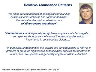
Relative-Abundance Patterns “No other general attribute of ecological communities besides species richness has commanded more theoretical and empirical attention than relative species abundance” “Commonness, and especially rarity, have long fascinated ecologists…, and species abundance is of central theoretical and practical importance in conservation biology…” “In particular, understanding the causes and consequences of rarity is a problem of profound significance because most species are uncommon to rare, and rare species are generally at greater risk to extinction” Photo of S. P. Hubbell from UCLA; quotes from Hubbell (2001, pg. 30)
Dominance-diversity (or rank-abundance) diagram, after Whittaker (1975) 1. Frequency histogram(Preston plot) Frequency (no. of spp.) Log10 abundance Log2 abundance Rank Relative-Abundance Patterns Empirical distributions of relative abundance (two graphical representations) Data from BCI 50-ha Forest Dynamics Plot, Panama; 229,069 individual trees of 300 species; most common species nHYBAPR=36,081; several rarest species nRARE=1
Relative-Abundance Patterns Approaches used to better understand relative abundance distributions 2. Mechanistic (deductive): Creating mechanistic models that predict the shapes of distributions 1. Descriptive (inductive): Fitting curves to empirical distributions A combined approach: create simple, mechanistic models that predict relative abundance distributions; adjust the model to maximize goodness-of-fit of predicted distributions to empirical distributions
Preston (1948) advocated log-normal distributions Log normal fit to the data 60 40 Number of species 20 1 16 256 4096 Log2 moth abundance (doubling classes or “octaves”) Figure from Magurran (1988)
Preston (1948) advocated log-normal distributions The left-hand portion of the curve may be missing beyond the “veil line” of a small sample Number of species 20 1 16 Log2 moth abundance (doubling classes or “octaves”) Figure from Magurran (1988)
Preston (1948) advocated log-normal distributions The left-hand portion of the curve may be missing beyond the “veil line” of a small sample 40 Number of species 20 1 16 256 Log2 moth abundance (doubling classes or “octaves”) Figure from Magurran (1988)
Preston (1948) advocated log-normal distributions The left-hand portion of the curve may be missing beyond the “veil line” of a small sample Log-normal fit to the data 60 40 Number of species 20 1 16 256 4096 Log2 moth abundance (doubling classes or “octaves”) Figure from Magurran (1988)
Variation among hypothetical rank-abundance curves Abundance (% of total individuals) Rank Figure from Magurran (1988)
Examples of relative-abundance data; each data set is best fit by one of the theoretical distributions broken-stick Abundance (% of total individuals) log-normal geometric series Rank Figure from Magurran (1988)
Log-normal distribution: Log of species abundances are normally distributed Why might this be so? May (1975) suggested that it arises from the statistical properties of large numbers and the Central Limit Theorem Central Limit Theorem: When a large number of factors combine to determine the value of a variable (number of individuals per species), random variation in each of those factors (e.g., competition, predation, etc.) will result in the variable being normally distributed J. H. Brown (1995, Macroecology, pg. 79): “…just as normal distributions are produced by additive combinations of random variables, lognormal distributions are produced by multiplicative combinations of random variables (May 1975)”
Abundance (% of total individuals) Rank Figure from Magurran (1988)
broken-stick Abundance (% of total individuals) log-normal geometric series Rank Figure from Magurran (1988)
Geometric series: The most abundant species usurps proportion k of all available resources, the second most abundant species usurps proportion k of the left-overs, and so on down the ranking to species S Does this seem like a reasonable mechanism, or just a metaphor with uncertain relevance to the real world? Sp. 4 … Sp. 3 Sp. 2 Sp. 1 Total Available Resources
Geometric series: This pattern of species abundance is found primarily in species-poor (harsh) environments or in early stages of succession broken-stick Remember, however, that pattern-fitting alone does not necessarily mean that the mechanistic metaphor is correct! Abundance (% of total individuals) log-normal geometric series Rank Figure from Magurran (1988)
Abundance (% of total individuals) Rank Figure from Magurran (1988)
broken-stick Abundance (% of total individuals) log-normal geometric series Rank Figure from Magurran (1988)
Broken Stick: The sub-division of niche space among species may be analogous to randomly breaking a stick into S pieces (MacArthur 1957) This results in a somewhat more even distribution of abundances among species than the other models, which suggests that it should occur when an important resource is shared more or less equitably among species Even so, there are not many examples of communities with species abundance fitting this model Sp. 5 Sp. 4 Sp. 3 Sp. 2 Sp. 1 Total Available Resources
Broken stick: Uncommon pattern In any case, remember that pattern-fitting alone does not necessarily mean that the mechanistic metaphor is correct! broken-stick Abundance (% of total individuals) log-normal geometric series Rank Figure from Magurran (1988)
Abundance (% of total individuals) Rank Figure from Magurran (1988)
Note the emphasis on rare species! Log series fit to the data Log normal fit to the data 60 40 Number of species 20 1 16 256 4096 Log2 moth abundance (doubling classes or “octaves”) Figure from Magurran (1988)
Log series: First described mathematically by Fisher et al. (1943) Log series takes the form: x, x2/2, x3/3,... xn/n where x is the number of species predicted to have 1 individual, x2 to have 2 individuals, etc... Fisher’s alpha diversity index () is usually not biased by sample size and often adequately discriminates differences in diversity among communities even when underlying species abundances do not exactly follow a log series You only need S and N to calculate it… S = * ln(1 + N/) But do we understand why the distribution of relative abundances often takes on this form? Photo of R. A. Fisher (1890-1962) from Wikimedia Commons
Hubbell’s Neutral Theory An attempt to predict relative-abundance distributions from neutral models of birth, death, immigration, extinction, and speciation Assumptions: individuals play a zero-sum game within a communityand have equivalent per capita demographic rates Immigration from a source pool occurs at random; otherwise species composition in the community is governed by community drift
Hubbell’s Neutral Theory Neutral model of local community dynamics Figure from Hubbell (2001)
Hubbell’s Neutral Theory Neutral model of local community dynamics Figure from Hubbell (2001)
Hubbell’s Neutral Theory Neutral model of local community dynamics Figure from Hubbell (2001)
Hubbell’s Neutral Theory An attempt to predict relative-abundance distributions from neutral models of birth, death, immigration, extinction, and speciation Assumptions: individuals play a zero-sum game within a communityand have equivalent per capita demographic rates Immigration from a source pool occurs at random; otherwise species composition in the community is governed by community drift The source pool (metacommunity) relative abundance is governed by its size, speciation and extinction rates Local community relative abundance is additionally governed by the immigration rate By adjusting these (often unmeasurable) parameters, one is able to fit predicted relative abundance distributions to those observed in empirical datasets
Hubbell’s Neutral Theory The model provides predictions that match nearly all observed distributions of relative abundance Theta () = 2JM JM = metacommunity size = speciation rate Figure from Hubbell (2001)
Hubbell’s Neutral Theory Model predictions can be fit to the observed relative-abundance distribution of trees on BCI Theta () = 2JM JM = metacommunity size = speciation rate m = immigration rate Figure from Hubbell (2001)
Hubbell’s Neutral Theory Does the good fit of the model to real data mean that we now understand relative abundance distributions mechanistically? Theta () = 2JM JM = metacommunity size = speciation rate m = immigration rate Figure from Hubbell (2001)
Barro Colorado Island 50-ha plot, Panama 7 topographically / hydrologically / successionally defined habitats Swamp1.20 ha Mixed2.64 ha Young1.92 ha Stream1.28 ha Low Plateau24.80 ha High Plateau6.80 ha Slope11.36 ha
Relative abundance is often a function of “Biology” 3355 total stems in the 1.2-ha swamp 171 species,each with > 60 stems
Relative abundance is often a function of “Biology” 303 species,each with at least 1 stem In 1990