Download
1 / 25
260 likes | 820 Vues
Statistics 111 - Lecture 13. Inference for a Population Mean. Confidence Intervals and Tests with unknown variance and Two-sample Tests . Administrative Notes. Homework 4 due Wednesday Homework 5 assigned tomorrow The final is ridiculously close (next Thursday). Outline. Review:

E N D
Statistics 111 - Lecture 13 Inference for a Population Mean Confidence Intervals and Tests with unknown variance and Two-sample Tests Stat 111 - Lecture 13 - One Mean
Administrative Notes • Homework 4 due Wednesday • Homework 5 assigned tomorrow • The final is ridiculously close (next Thursday) Stat 111 - Lecture 13 - One Mean
Outline • Review: • Confidence Intervals and Hypothesis Tests which assume known variance • Population variance unknown: • t-distribution • Confidence intervals and Tests using the t-distribution • Small sample situation • Two-Sample datasets: comparing two means • Testing the difference between two samples when variances are known • Moore, McCabe and Craig: 7.1-7.2 Stat 111 - Lecture 13 - One Mean
Chapter 5: Sampling Distribution of • Distribution of values taken by sample mean in all possible samples of size n from the same population • Standard deviation of sampling distribution: • Central Limit Theorem: • Sample mean has a Normal distribution • These results all assume that the sample size is large and that the population variance is known Stat 111 - Lecture 13 - One Mean
Chapter 6: Confidence Intervals • We used sampling distribution results to create two different tools for inference • Confidence Intervals: Use sample mean as the center of an interval of likely values for pop. mean • Width of interval is a multiple Z* of standard deviation of sample mean • Z* calculated from N(0,1) table for specific confidence level (eg. 95% confidence means Z*=1.96) • We assume large sample size to use N(0,1) distribution, and we assume that is known (usually just use sample SD s) Stat 111 - Lecture 13 - One Mean
Chapter 6: Hypothesis Testing • Compare sample mean to a hypothesized population mean 0 • Test statistic is also a multiple of standard deviation of the sample mean • p-value calculated from N(0,1) table and compared to -level in order to reject or accept null hypothesis • Eg. p-value < 0.05 means we reject null hypothesis • We again assume large sample size to use N(0,1) distribution, and we assume that is known Stat 111 - Lecture 13 - One Mean
Unknown Population Variance • What if we don’t want to assume that population SD is known? • If is unknown, we can’t use our formula for the standard deviation of the sample mean: • Instead, we use the standard error of the sample mean: • Standard error involves sample SD s as estimate of Stat 111 - Lecture 13 - One Mean
t distribution • If we have small sample size n and we need to use the standard error formula because the population SD is unknown, then: The sample mean does not have a normal distribution! • Instead, the sample mean has a T distribution with n - 1 degrees of freedom • What the heck does that mean?!? Stat 111 - Lecture 13 - One Mean
t distribution Normal distribution • t distribution looks like a normal distribution, but has “thicker” tails. The tail thickness is controlled by the degrees of freedom • The smaller the degrees of freedom, the thicker the tails of the t distribution • If the degrees of freedom is large (if we have a large sample size), then the t distribution is pretty much identical to the normal distribution t with df = 5 t with df = 1 Stat 111 - Lecture 13 - One Mean
Known vs. Unknown Variance • Before: Known population SD • Sample mean is centered at and has standard deviation: • Sample mean has Normal distribution • Now: Unknown population SD • Sample mean is centered at and has standard error: • Sample mean has t distribution with n-1 degrees of freedom Stat 111 - Lecture 13 - One Mean
New Confidence Intervals • If the population SD is unknown, we need a new formula for our confidence interval • Standard error used instead of standard deviation • t distribution used instead of normal distribution • If we have a sample of size n from a population with unknown , then our 100·C % confidence interval for the unknown population mean is: • The critical value is calculated using a table for the t distribution (back of textbook) Stat 111 - Lecture 13 - One Mean
Tables for the t distribution • If we want a 100·C% confidence interval, we need to find the value so that we have a probability of C between -t* and t* in a t distribution with n-1 degrees of freedom • Example: 95% confidence interval when n = 14 means that we need a tail probability of 0.025, so t*=2.16 = 0.95 df = 13 = 0.025 -t* t* Stat 111 - Lecture 13 - One Mean
Example: NYC blackout baby boom • Births/day from August 1966: • Before: we assumed that was known, and used the normal distribution for a 95% confidence interval: • Now: let be unknown, and used the t distribution with n-1 = 13 degrees of freedom to calculate our a 95% confidence interval: • Interval is now wider because we are now less certain about our population SD Stat 111 - Lecture 13 - One Mean
Another Example: Calcium in the Diet • Daily calcium intake from 18 people below poverty line (RDA is 850 mg/day) • Before: used known = 188 from previous study, used normal distribution for 95% confidence interval: • Now: let be unknown, and use the t distribution with n-1 = 17 degrees of freedom to calculate our a 95% confidence interval: Again, Wider interval because we have an unknown Stat 111 - Lecture 13 - One Mean
New Hypothesis Tests • If the population SD is unknown, we need to modify our test statistics and p-value calculations as well • Standard error used in test statistic instead of standard deviation • t distribution used to calculate the p-value instead of standard normal distribution Stat 111 - Lecture 13 - One Mean
Example: Calcium in Diet • Daily calcium intake from 18 people below poverty line • Test our data against the null hypothesis that 0 = 850 mg (recommended daily allowance) • Before: we assumed known = 188 and calculated test statistic T= -2.32 • Now: is actually unknown, and we use test statistic with standard error instead of standard deviation: Stat 111 - Lecture 13 - One Mean
Example: Calcium in Diet Normal distribution prob = 0.01 • Before: used normal distribution to get p-value = 0.02 • Now: is actually unknown, and we use t distribution with n-1 = 17 degrees of freedom to get p-value ≈ 0.04 • With unknown , we have a p-value that is closer to the usual threshold of = 0.05 than before T= -2.32 T= 2.32 t17 distribution prob ≈ 0.02 T= -2.26 T= 2.26 Stat 111 - Lecture 13 - One Mean
Review • Known population SD • Use standard deviation of sample mean: • Use standard normal distribution • Unknown population SD • Use standard deviation of sample mean: • Use t distribution with n-1 d.f. Stat 111 - Lecture 13 - One Mean
Small Samples • We have used the standard error and t distribution to correct our assumption of known population SD • However, even t distribution intervals/tests not as accurate if data is skewed or has influential outliers • Rough guidelines from your textbook: • Large samples (n> 40): t distribution can be used even for strongly skewed data or with outliers • Intermediate samples (n > 15): t distribution can be used except for strongly skewed data or presence of outliers • Small samples (n < 15): t distribution can only be used if data does not have skewness or outliers • What can we do for small samples of skewed data? Stat 111 - Lecture 13 - Means
Techniques for Small Samples • One option: use log transformation on data • Taking logarithm of data can often make it look more normal • Another option: non-parametric tests like the sign test • Not required for this course, but mentioned in text book if you’re interested Stat 111 - Lecture 13 - Means
Comparing Two Samples • Up to now, we have looked at inference for one sample of continuous data • Our next focus in this course is comparing the data from two different samples • For now, we will assume that these two different samples are independent of each other and come from two distinct populations Population 1:1 , 1 Population 2:2 , 2 Sample 1: , s1 Sample 2: , s2 Stat 111 - Lecture 13 - Means
Blackout Baby Boom Revisited • Nine months (Monday, August 8th) after Nov 1965 blackout, NY Times claimed an increased birth rate • Already looked at single two-week sample: found no significant difference from usual rate (430 births/day) • What if we instead look at difference between weekends and weekdays? Weekdays Weekends Stat 111 - Lecture 13 - Means
Two-Sample Z test • We want to test the null hypothesis that the two populations have different means • H0: 1 = 2 or equivalently, 1 - 2 = 0 • Two-sided alternative hypothesis: 1 - 2 0 • If we assume our population SDs 1 and 2 are known, we can calculate a two-sample Z statistic: • We can then calculate a p-value from this Z statistic using the standard normal distribution • Next class, we will look at tests that do not assume known 1 and 2 Stat 111 - Lecture 13 - Means
Two-Sample Z test for Blackout Data • To use Z test, we need to assume that our pop. SDs are known: 1 = s1 = 21.7 and 2 = s2 = 24.5 • We can then calculate a two-sided p-value for Z=7.5 using the standard normal distribution • From normal table, P(Z > 7.5) is less than 0.0002, so our p-value = 2 P(Z > 7.5) is less than 0.0004 • We reject the null hypothesis at -level of 0.05 and conclude there is a significant difference between birth rates on weekends and weekdays • Next class: get rid of assumption of known 1 and 2 Stat 111 - Lecture 13 - Means
Next Class – Lecture 14 • More on Comparing Means between Two Samples • Moore, McCabe and Craig: 7.1-7.2 Stat 111 - Lecture 13 - Means