Download

1 / 15
150 likes | 153 Vues
This section covers assumptions, distribution types, and calculations for inference about a population mean in AP Statistics.

E N D
Section 11.1Inference for the Mean of a Population AP Statistics
Inference for the Mean of a Population • If our data comes from a simple random sample (SRS) and the sample size is sufficiently large, then we know that the sampling distribution of the sample means is approximately normal with mean μ and standard deviation . • The spread of the sampling distribution depends on n and σ. σis generally unknown and must be estimated. • NOW…THEORY ASIDE AND ONTO PRACTICE ! AP Statistics, Section 11.1
Assumptions for Inference About a Mean • SRS – size n • Normal distribution of a population • μ and σare unknown • To estimate σ– use “S” in its place Then the standard errorof the sample mean is AP Statistics, Section 11.1
When σis known - • The z statistic has N (0,1) • When s is substituted the distribution is no longer normal AP Statistics, Section 11.1
The t statistic • The t statistic is used when we don’t know the standard deviation of the population, and instead we use the standard deviation of the sample distribution as an estimation. • The t statistic has n-1 degrees of freedom (df). AP Statistics, Section 11.1
The t statistic • Interpret the t statistic in the same way as the z statistic • There is a different distribution for every sample size. • The t statistic has n-1 degrees of freedom. • Write t (k) to represent the t distribution with k degrees of freedom. • Density curves for the t distribution are similar to the normal curve (symmetrical and bell shaped) • The spread is greater and there is more probability in the tails and less in the center. • Using s introduces more variability than sigma. • As d.f. increase, t(k) gets more normal AP Statistics, Section 11.1
The t statistic • In statistical tests of significance, we still have H0 and Ha. • We need to provide the mu in the calculation of the t statistic. • Looking at the t table is fundamentally different than the z table. AP Statistics, Section 11.1
One Sample t Confidence Intervals • Assume SRS size n with population mean μ • Confidence interval will be correct for normal populations and approx. correct for large n. AP Statistics, Section 11.1
Example: Mr. Young Mopping • Let’s suppose that Mr. Young has been told that he should mop the floor by 1:25 p.m. each day. • We collect 12 sample times with an average of 27.58 minutes after 1 p.m. and with a standard deviation of 3.848 minutes. • Find a 95% confidence interval for Mr. Young’s mopping times. AP Statistics, Section 11.1
Continued…. AP Statistics, Section 11.1
How about a 1 sample t-test?(A hypotheses test) Step 1: • Population of interest: • Mr. Young’s mopping time • Parameter of interest: • average time of arrival to mop • Hypotheses • H0: µ=25 min past 1:00 • Ha: µ>25 min past 1:00 AP Statistics, Section 11.1
Step 2: Mr. Young Mopping State type of test and conditions • We are using 1 sample t-test? • Bias? • SRS not stated. Proceed with caution. • Independence? • Population size is at least 10 times the sample size? • We assume that Mr. Young has mopped on a lot of days • Normality? • Big sample size (> 30). No • Sample is somewhat normal because the sample distribution is single peaked, no obvious outliers. AP Statistics, Section 11.1
Step 3: Mr. Young Mopping • Calculate the test statistic, and calculate the p-value from Table C AP Statistics, Section 11.1
Statistically Significant? • Is the t-value of 2.322 statistically significant at the 5% level? At the 1% level? • Does this test provide strong evidence that Mr. Young arrives on time to complete his mopping? Try this exercise on your calculator using: STAT TESTS Tinterval STAT TESTS T-Test AP Statistics, Section 11.1
Exercises • Wednesday: 11.6 – 11.11 • Thursday: 11.13 – 11.20 • Friday: T-Test Worksheet AP Statistics, Section 11.1