Download
1 / 17
170 likes | 248 Vues
Inference for the Mean of a Population. AP Stats Section 11.1. Getting Started. No longer given σ , which is a good thing! Process is slightly changed. Interpretation is still the same!. Some Basic Facts. Assumptions: Data is from a SRS

E N D
Inference for the Mean of a Population AP Stats Section 11.1
Getting Started • No longer given σ, which is a good thing! • Process is slightly changed. • Interpretation is still the same!
Some Basic Facts • Assumptions: • Data is from a SRS • Data come forma normal distribution where µ and σ are both unknown • OR • n ≥ 40 • Estimate σ with s, so always use (standard error)
Some Basic Facts • t – distributions: • Slightly different shape, based on sample size. • The larger the sample the closer to normal. (pg. 589) • Formulas • with a degree of freedom (df) = n -1 • What is a “degree of freedom?”
Confidence Intervals • Formula: • t* = upper critical value = • Need degree of freedom for t values • Ex: Turn to pg. 593 • Still using PANIC!
Confidence Intervals • P = parameter of interest is µ. • A = Can assume SRS for now. σ and µ are not known/given, sample is a little small • N = Using a t score: • I = Need to find all variables… • Plug the values into your calculator.
Confidence Intervals • Here they are: • s = 20.741 df = 4 t* = 2.776 • 44.44 ± 2.776(20.741/√5) • 44.44 ± 25.75 • 18.69 to 70.19 micrograms • We are 95% confident that the true mean amount of D-glucose in roaches after 10 hours is between 18.69 and 70.19micrograms .95
Hypothesis/ Significance Tests • Ho and Ha: still estimating µ, so no change here. • Test Stat; use new formula for t – score. • P – Value: use Table C to estimate where the p-value is, look within the table using the df. • Ex: Cola Sweetness pg. 594 • Are these data good evidence that the cola has lost sweetness? • Still using PHANTOMS!
Hypothesis/ Significance Tests • P = estimating µ • H = Ho: µ = 0 and Ha: µ >0 • A = can assume SRS, µ and σ unknown • N = using a t – score • T = • O = P – value: use df of 9 and look for 2.70
Hypothesis/ Significance Tests • It’s not there!! • P-Value is between .01 and .02. • M = Evidence to reject Ho • S= There is evidence to suggest that the cola has lost sweetness. • DONE!
Software Output • Let’s take a look at page 596…
Matched Pairs t • Situations: • Subjects are matched in pairs. Each treatment is given to one subject in each pair. • Before and After experiment on same subject (like cola) • **Population is actually the differences with in each matched pair! • The test is looking at the difference in responses. • This means Ho = 0 (Why?)
Matched Pairs t • Let’s do pg. 599 • Looking for a positive gain. • P= estimating µ • H = Ho: µ = 0 and Ha: µ >0 • A = can assume SRS, no µ or σ • N = Using a matched pairs t test • T =
Matched Pairs t • O = look for the p-value in Table C • P – value is between .0005 and .001 • M = Reject the Ho. • S = There is strong evidence that the teachers have gained understanding in the institute.
Matched Pairs t • Let’s do a 90% confidence Interval with the same problem… • P = estimating µ • A = OK • N= t – interval • I = t* = 1.729 2.5 ± 1.729(2.893/√20) 2.5 ± 1.12 1.38 to 3.62 points • C= We are 90% confident that the true average gain for teachers in the institute is between 1.38 and 3.62 points.
Robustness/Use of t • t procedures are only exactly correct when the population is normal. This rarely happens! • Robust: a confidence interval of sig test is robust if the confidence level or p – value don’t change very much when the assumptions are violated. • Check for outliers: they change the results and indicate a non-normal shape! • Make a graph first to check if it is alright to use t!
Rules to Know • Except when n is small (n < 15) it is more important to be a SRS than a normal distribution. • When n < 15, check for a close to normal distribution. If not close, or you have outliers, NO T IS ALLOWED! • When n ≥ 15, t is alright except with outliers of a strong skewed graph. • When n ≥ 40, t is always ok! (CLT)