Download
1 / 50
500 likes | 509 Vues
Inference on the Mean of a Population - Variance Known. &4-4 (&8-2). H 0 : m = m 0 H 1 : m m 0 , where m 0 is a specified constant. Sample mean is the unbiased point estimator for population mean. The Reasoning.

E N D
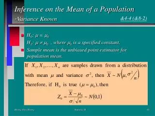
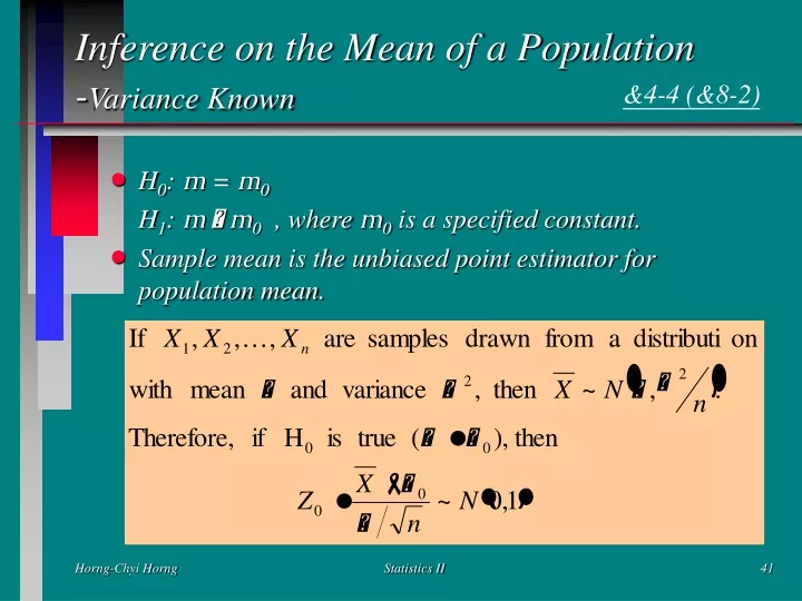
Inference on the Mean of a Population-Variance Known &4-4 (&8-2) • H0: m = m0 H1: m m0 , where m0 is a specified constant. • Sample mean is the unbiased point estimator for population mean. Statistics II
The Reasoning • For H0 to be true, the value of Z0 can not be too large or too small. • Recall that 68.3% of Z0 should fall within (-1, +1) 95.4% of Z0 should fall within (-2, +2) 99.7% of Z0 should fall within (-3, +3) • What values of Z0 should we reject H0? (based on a value) What values of Z0 should we conclude that there is not enough evidence to reject H0? Statistics II
Example 8-2 Aircrew escape systems are powered by a solid propellant. The burning rate of this propellant is an important product characteristic. Specifications require that the mean burning rate must be 50 cm/s. We know that the standard deviation of burning rate is 2 cm/s. The experimenter decides to specify a type I error probability or significance level of α = 0.05. He selects a random sample of n = 25 and obtains a sample average of the burning rate of x = 51.3 cm/s. What conclusions should be drawn? Statistics II
Hypothesis Testing on m- Variance Known Statistics II
P-Values in Hypothesis Tests(I) • Where Z0 is the test statistic, and (z) is the standard normal cumulative function. • In example 8-2, Z0 = 3.25, P-Value = 2[1-F(3.25)] = 0.0012 Statistics II
P-Values of Hypothesis Testing on m- Variance Known Statistics II
P-Values in Hypothesis Tests(II) • a-value is the maximum type I error allowed, while P-value is the real type I error calculated from the sample. • a-value is preset, while P-value is calculated from the sample. • When P-value is less than a-value, we can safely make the conclusion “Reject H0”. By doing so, the error we are subjected to (P-value) is less than the maximum error allowed (a-value). Statistics II
Type II Error- Fail to reject H0 while H0 is false Statistics II
How to calculate Type II Error? (I)(H0: m = m0 Vs. H1: mm0) • Under the circumstance of type II error, H0 is false. Supposed that the true value of the mean is m = m0 + d, where > 0. The distribution of Z0 is: Statistics II
How to calculate Type II Error? (II) - refer to section &4.3 (&8.1) • Type II error occurred when (fail to reject H0 while H0 is false) • Therefore, Statistics II
The Sample Size (I) • Given values of a and d, find the required sample size n to achieve a particular level of b.. Statistics II
The Sample Size (II) • Two-sided Hypothesis Testing • One-sided Hypothesis Testing Statistics II
Example 8-3 Statistics II
The Operating Characteristic Curves- Normal test (z-test) • Use to performing sample size or type II error calculations. • The parameter d is defined as: so that it can be used for all problems regardless of the values of m0 and s. • Chart VI a,b,c,d are for Z-test. Statistics II
Example 8-5 Statistics II
Large Sample Test • If n 30, then the sample variance s2 will be close to s2 for most samples. • Therefore, if population variance s2 is unknown but n 30, we can substitute s with s in the test procedure with little harmful effect. Statistics II
Large Sample Hypothesis Testing on m- Variance Unknown but n 30 Statistics II
Statistical Vs. Practical Significance • Practical Significance = 50.5-50 = 0.5 • Statistical Significance P-Value for each sample size n. Statistics II
Notes • be careful when interpreting the results from hypothesis testing when the sample size is large, because any small departure from the hypothesized value m0 will probably be detected, even when the difference is of little or no practical significance. • In general, two types of conclusion can be drawn: 1. At a = 0.**, we have enough evidence to reject H0. 2. At a = 0.**, we do not have enough evidence to reject H0. Statistics II
Confidence Interval on the Mean (I) • Point Vs. Interval Estimation • The general form of interval estimate is L m U in which we always attach a possible error a such that P(L m U) = 1-a That is, we have 1-a confidence that the true value of m will fall within [L, U]. • Interval Estimate is also called Confidence Interval (C.I.). Statistics II
Confidence Interval on the Mean (II) • L is called the lower-confidence limit and U is the upper-confidence limit. • Two-sided C.I. Vs. One-sided C.I. Statistics II
Construction of the C.I. • From Central Limit Theory, • Use standardization and the properties of Z, Statistics II
Formula for C.I. on the Mean with Variance Known • Used when 1. Variance known 2. n 30, use s to estimate s. Statistics II
Example 8-6 Consider the rocket propellant problem in Example 8-2. Find a 95% C.I. on the mean burning rate? 95% C.I => a = 0.05, za/2 = z0.025 = 1.96 Statistics II
Notes - C.I. • Relationship between Hypothesis Testing and C.I.s • Confidence level (1-a) and precision of estimation (C.I. * 1/2) • Sample size and C.I.s Statistics II
Choice of Sample Size to Achieve Precision of Estimation Statistics II
Example 8-7 Statistics II
One-Sided C.I.s on the Mean Statistics II
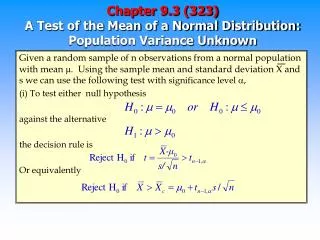
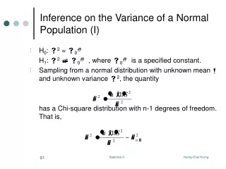
Inference on the Mean of a Population-Variance Unknown &4-5 (&8-3) • H0: m = m0 H1: m m0 , where m0 is a specified constant. • Variance unknown, therefore, use s instead of s in the test statistic. • If n is large enough ( 30), we can use the test procedure in &4-4 (&8-2). However, n is usually small. In this case, T0 will not follow the standard normal distribution. Statistics II
Inference on the Mean of a Population-Variance Unknown • Let X1, X2, …, Xn be a random sample for a normal distribution with unknown mean m and unknown variance s2. The quantity has a t distribution with n - 1 degrees of freedom. Statistics II
The Reasoning • For H0 to be true, the value of T0 can not be too large or too small. • What values of T0 should we reject H0? (based on a value) What values of T0 should we conclude that there is not enough evidence to reject H0? • Although when n 30, we can use Z0 in section &8-2 to perform the testing instead. We prefer using T0 to more accurately reflect the real testing result if t-table is available. Statistics II
Example 8-8 Statistics II
Testing for Normality (Example 8-8)- t-test assumes that the data are a random sample from a normal population (1) Box Plot (2) Normality Probability Plot Statistics II
Hypothesis Testing on m- Variance Unknown Statistics II
Finding P-Values • Steps: 1. Find the degrees of freedom (k = n-1)in the t-table. 2. Compare T0 to the values in that row and find the closest one. 3. Look the a value associated with the one you pick. The p-value of your test is equal to this a value. • In example 8-8, T0 = 4.90, k = n-1 = 21, P-Value < 0.0005 because the t value associated with (k = 21, a = 0.0005) is 3.819. Statistics II
P-Values of Hypothesis Testing on m- Variance Unknown Statistics II
The Operating Characteristic Curves- t-test • Use to performing sample size or type II error calculations. • The parameter d is defined as: so that it can be used for all problems regardless of the values of m0 and s. • Chart VI e,f,g,h are used in t-test. (pp. A14-A15) Statistics II
Example 8-9 • In example 8-8, if the mean load at failure differs from 10 MPa by as much as 1 MPa, is the sample size n = 22 adequate to ensure that H0 will be rejected with probability at least 0.8? s = 3.55, therefore, d = 1.0/3.55 = 0.28. Appendix Chart VI g, for d = 0.28, n = 22 => b = 0.68 The probability of rejecting H0: m = 10 if the true mean exceeds this by 1.0 MPa (reject H0 while H0 is false) is approximately 1 - b = 0.32, which is too small. Therefore n = 22 is not enough. At the same chart, d = 0.28, b = 0.2 (1-b=0.8) => n = 75 Statistics II
Construction of the C.I. on the Mean - Variance Unknown • In general, the distribution of is t with n-1 d.f. • Use the properties of t with n-1 d.f., Statistics II
Formula for C.I. on the Mean with Variance Unknown Statistics II
Example 8-10 Reconsider the tensile adhesive problem in Example 8-8. Find a 95% C.I. on the mean? • N = 22, sample mean = 13.71, s = 3.55, ta/2,n-1 = t0.025,21 = 2.080 13.71 - 2.080 (3.55) / 22 m 13.71 + 2.080 (3.55) / 22 13.71 - 1.57 m 13.71 + 1.57 12.14 m 15.28 The 95% C.I. On the mean is [12.14, 15.28] Statistics II
Final Note for the Inference on the Mean Statistics II