Download
1 / 16
180 likes | 841 Vues
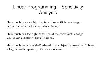
Linear Programming – Sensitivity Analysis. How much can the objective function coefficients change before the values of the variables change? How much can the right hand side of the constraints change you obtain a different basic solution?

E N D
Linear Programming – Sensitivity Analysis How much can the objective function coefficients change before the values of the variables change? How much can the right hand side of the constraints change you obtain a different basic solution? How much value is added/reduced to the objective function if I have a larger/smaller quantity of a scarce resource?
Linear Programming – Sensitivity Leo Coco Problem Max 20x1 + 10 x2 s.t. x1 - x2 <= 1 3x1 + x2 <= 7 x1, x2 >= 0 Solution: x1 = 0, x2 = 7 Z = 70 Issue: How much can you change a cost coefficient without changing the solution?
Sensitivity – Change in cost coefficient What if investment 2 only pays $5000 per share? Max 20x1 + 5 x2 s.t. x1 - x2 <= 1 3x1 + x2 <= 7 x1, x2 >= 0 New objective function isobar Optimal solution is now the point (2,1). Issue: At what value of C2 does solution change?
Sensitivity – Change in cost coefficient Issue: At what value of C2 does solution change? Ans.: When objective isobar is parallel to the binding constraint. Max 20x1 + C2* x2 s.t. 3x1 + x2 <= 7 3/1 = 20/C2 or C2 = 20/3 or 6.67
Sensitivity – Change in cost coefficient Lindo Sensitivity Analysis Output – Leo Coco Problem LP OPTIMUM FOUND AT STEP 1 OBJECTIVE FUNCTION VALUE 1) 70.00000 VARIABLE VALUE REDUCED COST X1 0.000000 10.000000 X2 7.000000 0.000000 ROW SLACK OR SURPLUS DUAL PRICES 1) 8.000000 0.000000 2) 0.000000 10.000000 NO. ITERATIONS= 1 RANGES IN WHICH THE BASIS IS UNCHANGED: OBJ COEFFICIENT RANGES VARIABLE CURRENT ALLOWABLE ALLOWABLE COEF INCREASE DECREASE X1 20.000000 10.000000 INFINITY X2 10.000000 INFINITY 3.333333 RIGHTHAND SIDE RANGES ROW CURRENT ALLOWABLE ALLOWABLE RHS INCREASE DECREASE 1 1.000000 INFINITY 8.000000 2 7.000000 INFINITY 7.000000
Sensitivity – Change in right hand side What if only 5 hours available in time constraint? Max 20x1 + 5 x2 s.t. x1 - x2 <= 1 3x1 + x2 <= 5 x1, x2 >= 0 New time constraint. Optimal solution is now the point (5,0). But, basis does not change. Issue: At what value of the r.h.s. does the basis change?
Sensitivity – Change in right hand side Issue: At what value of the r.h.s. does the basis change? Max 20x1 + 5 x2 s.t. x1 - x2 <= 1 3x1 + x2 <= ? x1, x2 >= 0 Basis changes at this constraint. x2 becomes non-basic at the origin. Or, when the constraint is: 3x1 + x2 < 0
Sensitivity – Change in right hand side Lindo Sensitivity Analysis Output – Leo Coco Problem LP OPTIMUM FOUND AT STEP 1 OBJECTIVE FUNCTION VALUE 1) 70.00000 VARIABLE VALUE REDUCED COST X1 0.000000 10.000000 X2 7.000000 0.000000 ROW SLACK OR SURPLUS DUAL PRICES 1) 8.000000 0.000000 2) 0.000000 10.000000 NO. ITERATIONS= 1 RANGES IN WHICH THE BASIS IS UNCHANGED: OBJ COEFFICIENT RANGES VARIABLE CURRENT ALLOWABLE ALLOWABLE COEF INCREASE DECREASE X1 20.000000 10.000000 INFINITY X2 10.000000 INFINITY 3.333333 RIGHTHAND SIDE RANGES ROW CURRENT ALLOWABLE ALLOWABLE RHS INCREASE DECREASE 1 1.000000 INFINITY 8.000000 2 7.000000 INFINITY 7.000000
Sensitivity – Shadow or Dual Prices Issue, how much are you willing to pay for one additional unit of a limited resource? Max 20x1 + 10 x2 s.t. x1 - x2 <= 1 (budget constraint 3x1 + x2 <= 7 (time constraint x1, x2 >= 0 Knowing optimal solution is (0,7) and time constraint is binding: Not willing to increase budget constraint (shadow price is $0). If time constraint increase by one unit (to 8), solution will change to (0,8) and Z=80. Therefore should be willing to pay up to $10(000s) for each additional unit of time constraint.
Sensitivity – Change in right hand side Lindo Sensitivity Analysis Output – Leo Coco Problem LP OPTIMUM FOUND AT STEP 1 OBJECTIVE FUNCTION VALUE 1) 70.00000 VARIABLE VALUE REDUCED COST X1 0.000000 10.000000 X2 7.000000 0.000000 ROW SLACK OR SURPLUS DUAL PRICES 1) 8.000000 0.000000 2) 0.000000 10.000000 NO. ITERATIONS= 1 RANGES IN WHICH THE BASIS IS UNCHANGED: OBJ COEFFICIENT RANGES VARIABLE CURRENT ALLOWABLE ALLOWABLE COEF INCREASE DECREASE X1 20.000000 10.000000 INFINITY X2 10.000000 INFINITY 3.333333 RIGHTHAND SIDE RANGES ROW CURRENT ALLOWABLE ALLOWABLE RHS INCREASE DECREASE 1 1.000000 INFINITY 8.000000 2 7.000000 INFINITY 7.000000
Linear Programming – Sensitivity Analysis What if more than one coefficient is changed?: 100% Rule (for objective function coefficients): if <= 1, the optimal solution will not change, where is the actual increase (decrease) in the coefficient and is the maximum allowable increase (decrease) from the sensitivity analysis.
Linear Programming – Sensitivity Analysis Example obj. function coefficient changes
Linear Programming – Sensitivity Analysis Simultaneous variations in multiple coefficients: 100% Rule (for RHS constants): if <= 1, the optimal basis and product mix will not change, where is the actual increase (decrease) in the coefficient and is the maximum allowable increase (decrease) from the sensitivity analysis.
Linear Programming – Sensitivity Analysis Example RHS constant changes
Linear Programming – Duality Theory Every LP has an associated dual problem. The Dual is essentially the inverse of the Primal (original problem). The optimal dual solution produces the dual price or shadow price reported in the Lindo output reports.
Integer Programming (IP) Similar to Linear Programming with the exception that decision variables must take on integer values. Drawbacks: solution effort considerably more difficult than Linear programming. Should we have used IP to solve the microwave oven homework problem? (solution was 147.8 model 1 and 100.0 model II ovens). Lindo solves both binary and integer programming problems.